Poisson-Approximation – Wikipedia

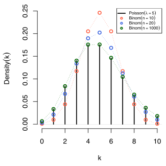
The Poisson-Approximation is a way in the probability calculation to approach the binomial distribution and the generalized binomial distribution for large samples and small probabilities through the Poisson distribution. The border crossing after infinitely infinitely gives the convergence in the distribution of the two binomial distributions against the Poisson distribution.

Is

${displaystyle (S_{n})}$

A sequence of binomial distributed random variables with parameters

${Displaystyle nin mathbb {n}}$

and

${displaystyle p_{n}}$

, so for the expectation values

$mms slepent It (Pys—Mi Phil.$

${displaystyle nto infty }$

applies, then follows

after-content-x4

${displaystyle p(S_{N}=k)=B_{N}}({k})to ,{frac {Lambda ^{k!}}mathrm {E} ^{-Lambda }=p_{Lambda }({k})Quad }$

for

${displaystyle nto infty }$

.

Evidence sketch [ Edit | Edit the source text ]

The value of a Poisson distributed random variable at the point

${displaystyle k}$

Is the limit

${displaystyle nto infty }$

a binomial distribution with

${displaystyle p={tfrac {lambda }{n}}}$

at the point

${displaystyle k}$

:

${displaystyle {begin{aligned}lim _{nto infty }P(S_{n}=k)&=lim _{nto infty }{binom {n}{k}}p^{k}(1-p)^{n-k}\&=lim _{nto infty }{frac {n!}{k!,(n-k)!}}left({frac {lambda }{n}}right)^{k}left(1-{frac {lambda }{n}}right)^{n-k}\&=lim _{nto infty }left({frac {lambda ^{k}}{k!}}right)left({frac {n(n-1)(n-2)cdots (n-k+1)}{n^{k}}}right)left(1-{frac {lambda }{n}}right)^{n}left(1-{frac {lambda }{n}}right)^{-k}\&={frac {lambda ^{k}}{k!}}cdot lim _{nto infty }underbrace {left({frac {n}{n}}cdot {frac {n-1}{n}}cdot {frac {n-2}{n}}cdots {frac {n-k+1}{n}}right)} _{to 1}underbrace {left(1-{frac {lambda }{n}}right)^{n}} _{to e^{-lambda }}underbrace {left(1-{frac {lambda }{n}}right)^{-k}} _{to 1}\&={frac {lambda ^{k}mathrm {e} ^{-lambda }}{k!}}.end{aligned}}}$

With large samples and small

${displaystyle p}$

The binomial distribution can therefore be accessible through the Poisson distribution.

The presentation as a limit of the binomial distribution allows an alternative calculation of the expectation value and variance of the Poisson distribution. Be

${Displaystyle x_ {1}, dotsc, x_ {n}, n}$

Independent Bernoulli distributed random variables

${Displaystyle, P = Lambda /N}$

and be

${Displaystyle s_ {n}: = x_ {1} +dotsb +x_ {n}}$

. For

${displaystyle nto infty }$

is applicable

${Displaystyle s_ {n} sim p_ {lambda}}}$

and

${displaystyle {begin{aligned}operatorname {E} (S_{n})&=operatorname {E} (X_{1})+dotsb +operatorname {E} (X_{n})=underbrace {{frac {lambda }{n}}+dotsb +{frac {lambda }{n}}} _{n,mathrm {mal} }=lambda to lambda \operatorname {Var} (S_{n})&=operatorname {Var} (X_{1})+dotsb +operatorname {Var} (X_{n})\&=underbrace {{frac {lambda }{n}}left(1-{frac {lambda }{n}}right)+dotsb +{frac {lambda }{n}}left(1-{frac {lambda }{n}}right)} _{n,mathrm {mal} }=lambda left(1-{frac {lambda }{n}}right)to lambda .end{aligned}}}$

Quality of the approximation [ Edit | Edit the source text ]

The following applies to the error assessment

${displaystyle sum _{kgeq 0}left|B_{n,p}({k})-P_{ncdot p}({k})right|leq 2np^{2}}$

.

The approximation of a sum of Bernoulli distributed random variables (or a binomial-distributed random variable) is therefore especially for small

${displaystyle p}$

good. As a rule of thumb, the approximation is good if

${displaystyle ngeq 50}$

and

${Displaystyle elder 0 {,} 05}$

is applicable. Is

${displaystyle papprox 0{,}5}$

So the normal ape proximation is more suitable.

generalization [ Edit | Edit the source text ]

The following can be shown more generally: are

${displaystyle X_{1},dotsc ,X_{n}}$

Stochastically independent random variables with

${displaystyle P(X_{i}=1)=p_{i}=1-P(X_{i}=0)}$

(Each random variable is therefore divided into Bernoulli). Then

${displaystyle S:=sum _{i=1}^{n}X_{i}}$

generalized binomial distributed and it is

${displaystyle lambda =sum _{i=1}^{n}p_{i}}$

.

Then apply

${displaystyle sum _{k=0}^{infty }left|P(S=k)-exp(-lambda ){frac {lambda ^{k}}{k!}}right|leq 2sum _{i=1}^{n}p_{i}^{2}}$

.

Is applicable

${displaystyle p_{i}=p_{j}}$

for all

${Displayt 1Leq i,jleq n}$

, so is

${displaystyle S}$

Distributed binomial and the above result follows immediately.

An individual of a species testifies

${displaystyle n=1000}$

Discussion, all of which stochastically independently of one another with a probability of

${displaystyle p_{i}=0{,}001}$

achieve sexual age. One is now interested in the probability that two or more descendants reach sexual age.

Exact solution [ Edit | Edit the source text ]

May be

${displaystyle X_{i}=1}$

The random variable “der

${displaystyle i}$

-Te descendant reaches the sexual maturity age ”. It applies

${displaystyle P(X_{i}=1)=p_{i}}$

and

${displaystyle P(X_{i}=0)=1-p_{i}}$

for all

${displaystyle i}$

. Then the number of survivors are offspring

${displaystyle S:=sum _{i=1}^{n}X_{i}}$

Because of the stochastic independence

${displaystyle B_{n,p}}$

-distributed.
The probability space is defined for modeling

${displaystyle (Omega ,Sigma ,P)}$

With the result quantity

${displaystyle Omega :={0,dotsc ,n}}$

, the number of surviving sexual tires. The σ algebra is then canonically the amount of potency of the result:

${displaystyle Sigma :={mathcal {P}}(Omega )}$

And as a distribution of probability the binomial distribution:

${displaystyle P({k}):=B_{n,p}({k})}$

.
Is looking for

${displaystyle P(Sgeq 2)=1-P(S=1)-P(S=0)=1-B_{1000;,0{,}001}({0})-B_{1000;,0{,}001}({1})approx 0{,}2642}$

. With a probability of approx. 26%, at least two individuals achieve sexual age.

Approximated solution [ Edit | Edit the source text ]

And

${displaystyle n}$

sufficiently large and

${displaystyle p}$

is sufficiently small, the binomial distribution can be reached sufficiently by means of the Poisson distribution. This time is the probability space

${displaystyle (Omega ,Sigma ,P)}$

defines using the result space

${displaystyle Omega :=mathbb {N} }$

, the

${displaystyle sigma }$

-Algebra

${displaystyle Sigma :={mathcal {P}}(mathbb {N} )}$

and the Poisson distribution as a probability distribution

${displaystyle p({K}):=p_{Lambda }({K})={Frac {lambada ^{K}} {K!},mathrm {E} ^{-lambada }}$

With the parameter

${displaystyle lambda =ncdot p=1}$

. Note here that the two modeled probability spaces are different, since the Poisson distribution on a finite result space does not define a probability distribution.
So the probability that at least two individuals achieve the sexual maturity age is

${displaystyle p(Sgeq 2 2)Approx 1-P_{Lambda }({1}})-p_{lambada }({0})=1-{frac {lambada ^{1}}{1!}}}e^E^-1————– 1}-{Frac {Lambda ^{0}}{0!}}e^{-1}}approx 0{,}2642}$

.

Except for four decimal places, the exact solution corresponds to the Poisson APPROPEPOPEOITION.

• Achim Klenke: Probability theory . 3. Edition. Springer-Verlag, Berlin Heidelberg 2013, ISBN 978-3-642-36017-6, DOI: 10,1007/978-3-642-36018-3 .
• Ulrich krengel: Introduction to probability theory and statistics . For studying, professional practice and teaching. 8. Edition. Vieweg, Wiesbaden 2005, ISBN 3-8348-0063-5, DOI: 10,1007/978-3-663-09885-0 .
• Hans-Otto George: Stochastics . Introduction to probability theory and statistics. 4th edition. Walter de Gruyter, Berlin 2009, ISBN 978-3-11-021526-7, DOI: 10.1515/9783110215274 .