Polymer in solution – Wikipedia

Understand the behavior of polymers in solution is important for certain applications such as cosmetic gels and creams. There is the possibility of controlling the viscosity of the product obtained and avoiding possible demixtion (phase separation). We note for example that the styrene is miscible in all proportion in the cyclohexane at 20 °C , but that when the styrene is polymized, there is no more miscibility. Different theories can explain these phenomena.

We model a polymer chain by a set of n links (monomer units) of volume a. The average number of links is linked to the degree of polymerization and the molar mass of the polymer. It is in solution in a solvent with a volume fraction or a known concentration.

Solvant polymer mixture [ modifier | Modifier and code ]

It is hypothesized that the molar volume of monomers units is equal to that of solvent molecules.
The mixture can be represented as this:

Flory-Huggins network representing the polymer in solution

At fixed temperature and pressure, the free mixture of mixture must be negative for the mixture to take place.
In the case of a regular solution, statistical thermodynamic calculations make it possible to estimate this free enthalpy:

${displaystyle delta g_ {m {acute {e}} l/site} = k_ {b} TCHI PHI (1-PHI)+K_ {b} t (phi ln (PHI)+(1-PHI) ln (1- PHI))}$

with

The Boltzmann constant, t la targeure in Kelvins,

the volume fraction and

A dimensionless parameter.

For a polymer in a solvent, Flory posed ^{[ first ]} :

${displaystyle delta g_ {m {acute {e}} l/site} = k_ {b} tchi ​​phi (1-PHI)+K_ {b} tleft ({frac {phi} {n}}}}}}}} 1-PHI) LN (1-PHI) RIGHT)}$

With n the average number of monomers per chain units.

This free enthalpy is actually the sum of two terms ^{[ 2 ]} :

${displaystyle Delta G_{m{acute {e}}l/site}=Delta H_{m{acute {e}}l/site}-TDelta S_{m{acute {e}}l/site}}$

Or :

${displaystyle Delta H_{m{acute {e}}l/site}}$

is the mixture of mixture;

${displaystyle Delta S_{m{acute {e}}l/site}}$

is the mixture of mixture, it is the latter which is decreased by factor N.

When n or the molar mass (it is equivalent) increases, entropy decreases, so disorder as well. There are indeed fewer possibilities to distribute the monomers units and the solvent molecules on the above grid when the chains are longer. The result is a free enthalpy of mixing more difficultly negative when the polymer has a stronger molar mass. This is in accordance with the precipitation that can be observed when you synthesize a polymer in solution, therefore in a solvent.

FLORY parameter [ modifier | Modifier and code ]

The parameter

which intervenes in the expression of the enthalpy and therefore in that of the free enthalpy, makes it possible to take into account the interactions between the polymer and the solvent. In this model ^{[ 3 ] , [ 4 ]} ,

${Displaystyle Text style chi = {frac {z} {k_ {b} t}} (epsilon _ {ms} -textstyle {1} {2}} (epsilon _ {mm}+epsilon _ {ss}))}$

Or :

Z is the number of first neighbors of monomeric units or solvent molecules;

${displaystyle scriptstyle epsilon _{MS}}$

is the interaction energy between monomer and solvent unit;

${displaystyle scriptstyle epsilon _{MM}}$

is the energy of interaction between monomers units;

${displaystyle scriptstyle epsilon _{SS}}$

is the interaction energy between solvent molecules.

This is Flory’s parameter, which plays an important role in the evolution of the free enthalpy:

When the florry parameter increases:

${displaystyle chi _{1}$

, a demixion zone appears and covers an increasingly large volume fractions range.

From a certain value of

, the curve has two inflection points and it is possible to draw a double tangent ^{[ 5 ]} . It is a sign of a separation in two phases like this ^{[ first ]} :

There is a demixion in 2 phases: one rich in polymer and the other poor, the volume fractions in polymer of the two phases are

${displaystyle phi _{R}}$

And

${Displaystyle Phi _ {p}}$

respectively.

We can calculate this critical value of Flory parameter ^{[ first ]} , noted

and obtained for

.

To summarize, the demixion appears when the Flory parameter exceeds a critical value which depends on the molar mass. This can also be understood by comparing the interactions that appear in the expression of this parameter. When

is tall,

dominated. This attractive energy is of course negative and when it is large, it decreases in absolute value: the attraction between polymer and solvent weakens. The links in polymer chains are attracted to each other and the polymer will be less and less solubilized.

We can access this flory parameter experimentally by osmotic pressure measurements for example.

State diagram

${displaystyle phi }$

-T [

${displaystyle phi }$

-T”>modifier |

${displaystyle phi }$

-T”>Modifier and code ]

For a polymer/solvent system, if the Van der Waals of London type interactions dominate (typically in the apolar environment), we can show that

varies as the reverse of the temperature. At low temperature, the Flory parameter will be large and we will have a demixion, and vice versa.

On the other hand when the hydrogen bonds dominate (polar environment),

Increases with temperature and we therefore have the opposite situation. At high temperature the thermal agitation breaks the hydrogen bonds which linked polymer to the solvent and the phase separation takes place.

To obtain these phase diagrams, we can start from tubes containing different molary fractions in polymer and observe when each tube becomes troubled when cooled from a temperature for which we mix ^{[ 6 ]} . The disorder is due to the diffusion of light in all directions by the particles which appear when the phase separation occurs:

Appearance of the disorder due to droplets which diffuse the light

Hildebrand approach, solubility parameter [ modifier | Modifier and code ]

We define the cohesion energy of the system and the cohesive energy density which is obtained by dividing the first by the molar volume ^{[ 6 ]} :

${DISPLAYSTYLE TEXTYLE C = {FRAC {Delta H_ {Vap} -RT}}}}}}}}}}}}}}}}}}}}}}}}}}}}}}}}}}}}}}}}}}}}}}}}}}}}}}}}}}}}}}}}}}}}}}}}}}}}}}}}}}}}}}}}}}}}}}}}}}}}}}}}}}}}}}}}}}}}}}}}}}}}}}}}$

.

The solubility parameter is then equal to the square root of this C density ^{[ 6 ]} :

${DisplayStyle Delta = Text style {sqrt {c}}}$

.

The solubility parameter values ​​are tabulated for many solvents and many polymers ^{[ 7 ]} . We can show that the Flory parameter seen previously can be written ^{[ 8 ]} :

${DisplayStyle chi = {frac {v_ {molar}} {rt}} (delta _ {solvent} -Delta _ {polym {grave {e}} re})^{2}}$

With R the perfect gas constant.
If we are looking for a good solvent for a given polymer, we must therefore seek a solubility parameter that is close to that of the polymer, to minimize the Flory parameter. We can thus eliminate many solvents for a given polymer, but even if Hildebrand’s parameters are close, the solubility is not ensured ^{[ 9 ]} .

We can also calculate the solubility parameter as this ^{[ 5 ]} :

${displaystyle delta ={frac {rho }{M}}sum _{i}G(i)}$

where G (i) is the molar attraction constant of group I ^{[ 7 ]} .

Let two compartments are separated by a semi permeable membrane:

Osmotic pressure illustration

The right compartment contains the polymer in solution in a solvent, while the left compartment contains only the solvent. We observe a variation in the pressure between the 2 compartments. More specifically, polymer chains exercise a force on the wall. This strength per unit of surface is called osmotic pressure . It can be calculated for a few hypotheses from the mixture of mixture seen previously.

If the volume fraction in polymer is not too large, we get:

${displaystyle pi ={frac {k_{B}T}{a^{3}}}left({frac {phi }{N}}+{frac {phi ^{2}}{2}}(1-2chi )right)}$

.

We realize that the value of the Flory parameter here still plays a role:

The Flory parameter

varies with temperature. When it takes the limit value 1/2, the associated temperature bears the name of “Théta temperature”. This particular temperature can often be in tables for a polymer/solvent torque. For example, cyclohexane is a polystyrene tea solvent ^{[ 5 ]} to 307.2 K.

This theory introduces the concept of excluded volume: there is a repulsion between chains, of a geometric nature, which prohibits the presence of the center of mass of another polymer chain around a given chain.

Modeling of the distribution of channels taking into account the excluded volume

The previously calculated florry parameter is changed ^{[ 11 ]} :

${DisplayStyle chi = chi _ {enthalpique; pr {acute {e}} c {acute {e}} tooth}+chi _ _ {entropique; from; in; volume; excluded}}$

.

With a polymer – solvent torque, we can associate a temperature

and a parameter

it Entropic parameter , both independent of the temperature ^{[ 11 ]} :

${displaystyle 1/2-chi =psi left(1-{frac {theta }{T}}right)}$

.

Knowing the critical temperature

(of the appearance of the disorder) for samples of a polymer of different molar masses, we can graphically determine the temperature

and the entropic parameter.

The excluded volume (U), the Flory parameter and the second viriel coefficient of the Polymer/Solvant A2 couple are linked by the following relations:

${displaystyle A_{2}=left({frac {1}{2}}-chi right)left({frac {N_{a}N^{2}a^{3}}{M^{2}}}right)={frac {Na,u}{2M^{2}}}}$

.

Na is the number of avogadro, n the number of segments, m the molar mass and has the volume of a monomer unit.

When the flory parameter is less than 0.5, the excluded volume increases: there is extension of the chains and we are in a good solvent diet. In bad solvent it is the opposite, there is a contraction of the channels. We can experimentally obtain the volume excluded by osmometry ^{[ twelfth ]} .

There are different regimes, depending on the concentration and mass of the polymer in solution. For entropic reasons, polymer channels are not unfolded but they contract on themselves to form balls.

Of the diluted diet with a semi -diluted diet [ modifier | Modifier and code ]

Be polymer balls in solution. When the concentration (or the volume fraction is increased which amounts to the same), the distance between balls decreases. From a moment, there is contact between the latter and we call Critical recovery concentration the associated concentration. It marks the transition between the diluted regime and the Semi diluted diet . It is still possible to increase the concentration in the semi -diluted diet, because the fraction of polymer contained in a ball is really low.

Effect of an increase in concentration on polymer balls in solution

We can calculate the critical recovery concentration using the following relation ^{[ 3 ] , [ 13 ]} :

${displaystyle C^{star }={frac {M_{W}}{{frac {4}{3}}Pi R_{g}^{3}N_{a}}}}$

.

The volume fraction depends on the number of segments of the channels to power -4/5.

Giration radius in diluted regime [ modifier | Modifier and code ]

This distance has an influence on the physicochemical properties of the system.
In good solvent ^{[ 6 ]} :

${displaystyle R_{g}mathbb {s} a.N^{3/5}}$

,

With RG the gimal radius of the balls and n the number of segments of the chain which constitutes the ball and is the size of these segments.
Solvent

:

${displaystyle R_{g}mathbb {s} a.N^{1/2}}$

.

We can understand this difference of exponent by taking into account the fact that by good solvent

, the repulsive interactions between segments of balls dominate. The balls swell and their radius of giration increases.

Solvent

, there are different models to calculate the giration radius:

• Random walking model ^{[ 2 ]} :
  ${Displaystyle ^{2}=N.a^{2}}$

  [ 6 ] ^{, [ 14 ]} :

${Displaystyle ^{2} = n.a^{2} {fraud {1+cos (Theta)} {1-Cos (Theta)}}}}$

${displaystyle theta }$

is the angle of Valence, taken according to this convention:

• Embarrassed rotation: we take into account the interactions between molecular groups.

${Displaystyle ^{2}=N.a^{2}{frac {1+cos(theta )}{1-cos(theta )}}{frac {1+cos(phi )}{1-cos(phi )}}}$

${displaystyle phi }$

is the internal rotation angle or dihedral angle. You can see

${displaystyle cos(phi )}$

like a rigidity coefficient.

If we are no longer in conditions

${displaystyle theta }$

, we can introduce a coefficient of volume expansion like this ^{[ 15 ]} :

${Displaystyle ^{2}=alpha ^{2}. _{theta }^{2}}$

Characteristic size in semi -diluted regime [ modifier | Modifier and code ]

When the balls interpenetrate, we can no longer really speak of a radius of gimal, since we cannot distinguish the balls. We define the average distance between tangle points, noted

${Displaystyle XI}$

. This quantity is equal to

${displaystyle R_{g}}$

When we are at the critical concentration of recovery. It then decreases when the concentration increases. The properties of the system depend on this quantity in the semi -diluted diet. We can show that ^{[ 2 ]} :

${displaystyle xi mathbb {S} aphi ^{-3/4}}$

As a good solvent.

${Displaystyle XI}$

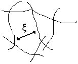is a correlation length, or network mesh.

The tangled diet [ modifier | Modifier and code ]

It is possible when the mass exceeds a critical mass of tangle MC. It can appear in the semi -diluted diet, even in the concentrated diet (when the concentration is even increased).
In the tangled diet, the movement of the chains is very embarrassed by that of the other chains. Its movement is described by the reputation model. The viscosity then depends on the concentration of 3.75 power and the mass in the cube. In a non -tangled diet, the viscosity depends on the concentration of only 2.5 power and the chains have a so -called “rouse” dynamic. This more or less large effect of concentration makes it possible to play on the viscosity of the system in a significant way and can be used when making polymer gels.

There are different techniques to study polymers in solution:

• Colligative thermodynamic methods:
• Viscosimetric methods:
  • Access to viscosity, the average viscosimetric molar mass ^{[ 6 ]} (Mn
• hydrodynamic techniques:
  • These, access to mass molar masses in mass and moles;
• light diffusion techniques:

1. ↑ ^{A B and C} Menno A. van Dijk and André Awake , Concepts of polymer thermodynamics , CRC Press, 1997 , 209 p. (ISBN  1-56676-623-0 And 9781566766234 , read online )
2. ↑ ^{A B and C} D ESPINAT , Application of light diffusion techniques, X -rays and neutrons to study colloidal systems , Paris, Technip editions, 1992 , 131 p. (ISBN  2-7108-0617-7-7 And 9782710806172 , read online )
3. ↑ ^{a et b} Hans-Georg Elias , Macromolecules : Volume 3 : Physical Structures and Properties , Wiley-VCH, 2008 , 699 p. (ISBN  978-3-527-31174-3 And 3-527-31174-2 , read online )
4. ↑ Some authors define it with Z-2 rather than Z.
5. ↑ ^{A B C and D} J. M. G. Cowie , Polymers : chemistry and physics of modern materials , CRC Press, 1991 , 436 p. (ISBN  0-7487-4073-2 And 9780748740734 , read online )
6. ↑ ^{a b c d e f g h and 1} Hans-Henning Cock , Nicole Heymans , Christopher-John Plummer and stone Decroly , Polymers’ materials: mechanical and physical properties, [Principles of implementation] , Lausanne/Paris, ppur Polytechnic presses, 2001 , 657 p. (ISBN  2-88074-415-6 And 9782880744151 , read online )
7. ↑ ^{a et b} Hildebrand parameter values ​​and molar attractions constants
8. ↑ Jean Vidal , Thermodynamics: Application to chemical engineering and the petroleum industry , Paris, Technip editions, 1997 , 500 p. (ISBN  2-7108-0715-7-7 And 9782710807155 , read online )
9. ↑ Andreĭ aleksandrovich Askadskiĭ , Physical properties of polymers : prediction and control , CRC Press, 1996 , 336 p. (ISBN  2-88449-220-8 And 9782884492201 , read online )
10. ↑ (in) MICHIO Kurata ( trad. Japanese), Thermodynamics of polymer solutions , Chur/London/New York, Taylor & Francis, 1982 , 294 p. (ISBN  3-7186-0023-4 And 9783718600236 , read online )
11. ↑ ^{a et b} Yuri S. Lipatov and anatoly E. Nesterov , Thermodynamics of polymer blends , CRC Press, 1997 , 450 p. (ISBN  1-56676-624-9 And 9781566766241 , read online )
12. ↑ Paul C. Hiemenz , Polymer chemistry : the basic concepts , CRC Press, 1984 , 738 p. (ISBN  0-8247-7082-X And 9780824770822 , read online )
13. ↑ Some authors define it with a 0.74 multiplicative coefficient in the numerator.
14. ↑ If we take another convention to define the angle, the formula is reversed.
15. ↑ English lesson