Continuous fraction – Wikipedia

In mathematics, a fraction continue or fraction continue simple or more rarely continued fraction ^{[ first ]} is an expression of the form:

with a finished or infinite number of stages.

We show that we can “represent” – in a sense which will be specified – any real number in the form of a continuous, finished or infinite fraction, in which a ₀ is a relative integer and the others a _j are strictly positive integers.

As in the usual decimal notation, where each real is approached by decimal numbers increasingly precisely as the data of successive decimals progresses, so each real is approached by stored fractions of the above form of above More and more precisely as we add floors. In addition, if it takes an infinity of decimal to describe exactly an uncimal number, an infinite development is needed in continuous fraction to describe exactly an irrational number.

Continuous fractions are useful in Diophantian approximation, in particular because they provide, in a certain sense, the “best” approximations of the real by rational. This property is at the origin of algorithms for the approximation of square roots, but also of demonstrations of irrationality or even transcendence for certain numbers such as Pi or It is . The periodicity of continuous fractions of the square roots of integers strictly greater than 1 and without square factor has useful consequences for the study of the Pell-Fermat equation.

Already used in Indian mathematicians in the Middle Ages, continuous fractions are studied in Europe from the XVII ^{It is} century. They are now generalized to other expressions, applied to the approximations of entire series called approximating of Padé, or even adapted to linear applications.

The notion of continuous fraction is vast and is found in many branches of mathematics. Associated concepts can be relatively simple such as euclide algorithm, or much more subtle such as that of meromorphic function ^{[ note 1 ]} .

It is possible, at first, to see a continuous fraction as a series of whole which “represents” a real. This situation is a bit the same as that of the decimal system which represents Pi Subsequently of integers 3, 1, 4, 1, 5, 9… in the form of a continuous fraction, the continuation is 3, 7, 15, 1, 292, 1, 1, a first field of study consists in studying The relationship between suite 3, 7, 15, 1, 292, 1, 1… and that of the rational numbers offered by the continuous fraction, in this case 3, 22/7, 333/106, etc., it allows you to Know how to go from the first following to the second, how the second converges and answers other questions of this nature. This is essentially the object of this article.

Continuous fractions have a particular relationship with square roots or more generally the numbers, so -called quadratic irrational, of the form

Or

And

are rational numbers,

not zero, and

[ 2 ] . This situation is like the infinite decimal representations of rational numbers. These continuous fractions make it possible to solve a famous arithmetic problem called Pell-Fermat equation ^{[ 3 ]} . This question is the subject of the article “continuous fraction of an irrational quadratic”.

Like the decimal system, the continuous fraction offers increasingly approached rational numbers of their target. These approximations are much better than decimal those. The second decimal approximation of Pi , equal to 31/10 has a denominator relatively close to that of the second approximation of the continuous fraction 22/7, on the other hand 22/7 is more than 30 times more precise than 31/10. This type of approach to a real number by a rational number is called Diophantian approximation. Continuous fractions play a big role there. They made it possible to build the first known transcendent numbers: the numbers of Liouville ^{[ 4 ]} or show that the number It is is irrational ^{[ 5 ]} . Provided to generalize the definition of a continuous fraction, it becomes possible to show that Pi is also irrational – this approach is treated in the article “Continuous fraction and Diophantian approximation”. (Actually, It is And Pi are even transcendent, according to Hermite-Lindemann’s theorem.)

A continuous fraction does not only concern numbers but also functions. We generalize the continuous fractions even more by replacing the coefficients with polynomials ^{[ 6 ]} . A motivation comes from the complex analysis, which aims to study the functions of the complex variable with complex values, derivable as such. The classic approach is to define them as whole series therefore as limits of polynomials. A frequent specificity of this type of function is to have poles. If, instead of approaching the function by polynomials, we use quotients, we build a series of approximents of pads which does not necessarily have this weakness ^{[ 7 ]} .

Other properties have been studied. Unlike the decimal system, an integer appearing in a continuous fraction is generally not limited by 9, it can become arbitrarily large. Alexandre Khintchine was interested in the average, in the sense of limit of the geometric averages of all these denominators. For almost all numbers, this average is the same (the word “almost” has here the technical meaning of measurement theory); This average is called Khintchine constant.

It is also possible to build developments in fractions by placing the fraction bars on the numerator and not below: we obtain a series development of Engel:

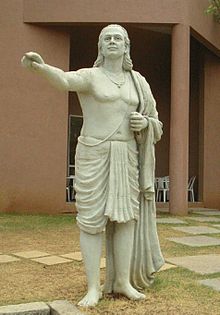
The use of continuous fractions is old. Aryabhata (476-550), an Indian mathematician uses them to resolve Diophantian equations as well as to approximately approximate irrational numbers ^{[ 8 ] [Ref. incomplete]} . Brahmagupta (598-668) studies the equation now so-called Pell-Fermat, using a remarkable identity. He seeks to solve the equation x ² – sixty one and ² = 1 and find the smallest solution: x = 1,766 319 049 and and = 226 153 980.

At XII ^{It is} century, the method is enriched by BHāskara II. An algorithm, the Chakravala method, similar to that of continuous fractions, makes it possible to resolve the general case ^{[ 9 ]} . The most striking difference with the subsequent European method is that it allows negative numbers in the fraction, allowing faster convergence ^{[ ten ]} .

The appearance in Europe is later and Italian. Raphaël Bombelli (1526-1572) uses an ancestor of continuous fractions for the calculation of approximations of the square root of 13 ^{[ 11 ]} . Pietro Cataldi (1548-1626) includes that the Bombelli method applies for all square roots, it uses it for value 18 and writes a small pamphlet on this subject ^{[ twelfth ]} . He notes that the approximations obtained are alternately higher and lower than the square root.

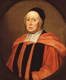
Decisive progress takes place in England. On January 3, 1657, Pierre de Fermat challenged European mathematicians with several questions including the equation already resolved by Brahmagupta ^{[ 13 ]} . The reaction of the English, stung ^{[ 14 ]} , is fast. William Brouncker (1620-1684) finds the relationship between the equation and the continuous fraction, as well as a algorithmic method equivalent to that of the Indians for the calculation of the solution. It produces the first generalized continuous fraction, for the number 4/π ^{[ note 2 ]} . These results are published by John Wallis who takes the opportunity to demonstrate the recurrence relations used by Brouncker and BHāskara II. It gives the name of fraction continue in the sentence : “Namely, if the unit is adjoining a fraction of which the denominator has Continue fractured ^{[ 15 ]} » . At that time, Christian Huygens (1629-1695) used the rational approximations given by the development in continuous fractions to determine the number of teeth of the gears of a planetary automaton ^{[ 16 ]} .

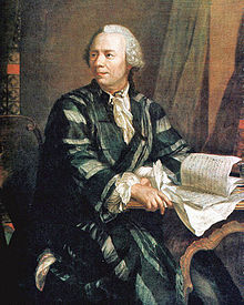
Some theoretical questions are resolved in the following century. The use shows that the algorithm of continuous fractions makes it possible to resolve the equation of Pell-Fermat using the fact that the fraction is periodic from a certain rank. Leonhard Euler (1707-1783) shows that if a number has a periodic continuous fraction, then it is a solution of a second degree equation with whole coefficients ^{[ 17 ]} . The reciprocal, more subtle ^{[ 18 ]} , is the work of Joseph-Louis Lagrange (1736-1813). During this century, Jean-Henri Lambert (1728-1777) found a new use for continuous fractions. He uses them to show the irrationality of Pi .

This use becomes frequent at XIX ^{It is} century. Evariste Galois (1811-1832) finds the necessary and sufficient condition for a continuous fraction to be immediately periodic ^{[ note 3 ]} . Joseph Liouville uses continuous fraction development to exhibit transcendent numbers: Liouville numbers ^{[ 4 ]} . In 1873, Charles Hermite proved the transcendence of It is . A by-product of its evidence is a new demonstration of the expression of the simple continuous fraction of It is found by Euler ^{[ 19 ]} . At the end of the century, Henri Padé (1863-1953) developed the theory ^{[ 20 ]} Approximants who now bear its name and which are continuous fractions of polynomials. This technique is used by Henri Poincaré (1854-1912) to demonstrate the statibilité ^{[That’s to say ?]} solar system ^{[ 21 ]} . Georg Cantor (1845-1918) proves using continuous fractions that the points of a segment and those located inside a square are in bijection ^{[ 22 ]} . The functions of this nature are studied within the framework of chaos theory; They are discontinuous on each rational point of the interval [0, 1] ^{[ 23 ]} .

From the euclide algorithm to continuous fractions [ modifier | Modifier and code ]

We start by recalling the course of the algorithm due to the PGCD research euclides, by analyzing the example of the two whole numbers 15,625 and 6,842. We proceed to a series of Euclidean divisions with rest:

Another way of interpreting this algorithm is to approach in stages the quotient 15 625/6 842. The whole part of this quotient is 2, which allows to write:

What can we say about fraction 1 941/6 842, except that it is smaller than 1? It is between 1/4 and 1/3, its inverse, 6,842/1 941, has as the whole part: 3; And more specifically, if we use the results of the second Euclidean division:

So step by step:

which is a continuous fraction. We sometimes use the following notation, more convenient:

15,625/6 842 can be compared to its reduced reduced by successively truncating the number of stages of the continuous fraction. The following table gives the truncations in fractional notation and then decimal, and the difference between the reduced and the number 15 625/6 842.

The rest of the errors is decreasing in absolute value and alternating signs.

Continuous fraction development of a rational [ modifier | Modifier and code ]

Either r = p / q a rational number (with p And q whole and q > 0). We are looking for r and finished development in continuous fraction , that is to say a writing of r Under the form [ a ₀ , …, a _n ] with n whole natural, a ₀ relative integer and a _first , …, a _n whole> 0. For this we apply the euclide algorithm:

On pose p ₀ = p , p _first = q , and we build whole a ₀ And p ₂ By Euclidean division:

Then, as long as p _j is not zero, we define the whole a _{j -first} And p _{j +1} about :

with a _{j -first} integer at least equal to 1 (for j > 1) and 0 ≤ p _{j +1} < p _j . The euclide algorithm stops. We notice n the largest whole for which p _{n +1} is not zero. So we know that p _n / p _{n +1} is equal to the whole a _n . We then have:

In effect :

or :

Geometric representation ^{[ 24 ]} –

A paving of a rectangle of length 30 and width 13 makes it possible to determine the expression of 30/13 in continuous fraction: 30/13 = [2, 3, 4].

The euclid algorithm makes it possible to calculate a continuous fraction in the case of rational numbers. This algorithm admits in this context a geometric interpretation. Either r = p / q a rational number, we consider a rectangle of length p and width q , and we pave it by side squares q .

And r is an integer, the pavingaux has exactly r squares. Otherwise, be a ₀ The number of squares inserted in the rectangle, or even the first term of the continuous fraction. There remains an unpaved band of dimension q × b _first with b _first equal to p – a ₀ q ; We pave this band with squares of maximum dimension, that is to say aside b _first . The number of squares is equal to the second term a _first continuous fraction. By reiterating the method, we obtain all of the coefficients a _p .

In the image opposite, we pave the 30 × 13 rectangle by two squares on sides 13. There remains a strip of length 13 and width 4. In terms of continuous fraction, we obtain equality:

${displaystyle {frac {30}{13}}=2+{frac {4}{13}}={color {Red}2}+{cfrac {1}{left({cfrac {13}{4}}right)}}}$

.

The same approach applies to determine a rational knowing its continuous fraction. [1, 1, 2, 3] = October 17

Then, we note that it is possible to fill the remaining band with 3 squares with side 4 and there remains a strip of length 4 and of width 1, which allows to finish the calculation of the continuous fraction:

${displaystyle 13=3times 4+1;Rightarrow ;{frac {30}{13}}={color {Red}2}+{cfrac {1}{left({cfrac {3times 4+1}{4}}right)}}={color {Red}2}+{cfrac {1}{{color {Red}3}+{cfrac {1}{color {Red}4}}}}=[2,3,4]}$

.

The paving technique leads to an infinite continuous fraction if the length and width of the rectangle are immeasurable.

The same construction makes it possible to find the rational whose development is known in continuous fraction. In the image of the left one can find the rational whose development is [1, 1, 2, 3]. The last coefficient is equal to 3, there are therefore 3 small squares side 1, which give the size of the next square (3). The penultimate coefficient 2 indicates that there are two medium squares on the side 3. These two sides and the small square give the size of the larger square (7). The associated coefficient is equal to 1, there is therefore only one unique of this nature. The larger square (7) and the average square (3) give the side of the last square (10). The last two squares give the total length of the rectangle (17). The desired fraction is equal to 17/10.

The process stops because p And q are commensurable, that is to say that there is a length l and two integers a And b such as p = the And q = lb .

Now consider a length rectangle L and width l . If the quotient L / l is not rational, that is to say if the lengths L And l The process is not immeasurable.

This is the case for the right figure representing a gold rectangle, that is to say a rectangle whose ratio of length on the width is equal to φ the golden number. We can only place a square in each band which leads to the representation:

${displaystyle varphi =[1,1,1,cdots ]}$

.

The rest of the numerators and that of the denominators are fibonacci.

We have therefore shown that for any rational r , the euclid algorithm provides a finite development in continuous fraction of r (Conversely, any number which has a finished development in continuous fraction is obviously rational). Development [ a ₀ , …, a _n ] thus obtained has the particularity if n is not zero, then a _n > 1. We deduce a second development: r = [ a ₀ , …, a _n – 1, 1]. These are the only two ^{[ 25 ] , [ 26 ]} .

When we add to the calculation of a _j of this development, the calculation of numerators h _j and denominators k _j Different reduced:

This euclide algorithm becomes the extensive euclide algorithm ^{[ 27 ] [Source diverted]} . More specifically, the continuation of couples of whole ( in _i , in _i ), provided by the extended algorithm applied to ( p , q ), coincides with the suite ( k _j , h _j ), to the signs of the nearest and a gap near the indices: k _j = (–1) ^j in _{j +2} And h _j = (–1) ^{j +1} in _{j +2} . For everything j , whole k _j And h _j are therefore primary between them and p _{j +1} = (–1) ^j ( QH _{j -first} – pk _{j -first} ). In particular: the last reduced, h _n / k _n , is the fraction p / q Iroductible form and the penultimate corresponds to the particular solution of the identity of Bézout supplied by the extended euclide algorithm: PGCD (PGCD ( p , q ) = p _{n +1} = (–1) ⁿ ( QH _{n -first} – pk _{n -first} ).

Development in continuous fraction of the number Pi [ modifier | Modifier and code ]

A note makes it possible to generalize the previous method to any real. To illustrate it, let’s apply it to the number Pi . The first step, in the case of a rational, was the calculation of the quotient of the Euclidean division of the numerator by the denominator, which no longer makes sense for a real, on the other hand the result was equal to the entire part of the rational, or the whole part of a real has a meaning. The fractional part, necessarily smaller than 1, was reversed, which is still possible here. We obtain :

As II – 3 is smaller than 1 (it is a fractional part) its inverse is larger than 1, and is not whole since Pi is irrational. We can therefore apply the same approach to him:

The new value, approximately equal to 15.997, is still an irrational strictly greater than 1, hence the possibility of a new step, then a new one:

Due to the fact that Pi is irrational, the process never stops (imagining that the calculation is carried out with an infinity of decimal). We obtain as a suite of fractions 3 then 22/7 ≈ 3.1428 then 333/106 ≈ 3.14150 then 355/113 ≈ 3.1415929 and finally 103 993/33 102, close to Pi With a better precision than the billionth. Once again, the rest of the errors is decreasing in absolute value and alternating signs.

Notations and terminology [ modifier | Modifier and code ]

• We will call fraction continue or fraction continue simple ^{[ note 4 ]} Any not empty ( a _p ) of which the first term a ₀ is a relative integer and all the following terms are strictly positive integers. ^{[ Ref. desired]}
• All of its indices is either in form {0, 1,…, n } for a certain natural integer n If it is a finished suite, either equal to ℕ for an infinite suite.
• on scaled down index p is the rational [ a ₀ , a _first , …, a _p ], defined by
  ${displaystyle [a_{0}]=a_{0},quad [a_{0},a_{1}]=a_{0}+{frac {1}{a_{1}}},quad dots [a_{0},dots ,a_{p}]=a_{0}+{frac {1}{[a_{1},dots ,a_{p}]}}.}$

  

Reduced by a continuous fraction [ modifier | Modifier and code ]

Either ( a _p ) a continuous fraction. We associate two whole suites ( h _p ) And ( k _p ), defined by recurrence by:

So, for any index p continuous fraction:

The property (3) shows, by application of the Bézout theorem, that the whole h _p And k _p are first between them.

These three properties are demonstrated directly ^{[ 28 ]} But are also special cases of those of generalized continuous fractions, demonstrated in the corresponding article. We also give a matrix interpretation of the definition of h _p And k _p , which follows immediately, by transposition, a dual property of (1) ^{[ 29 ]} :

${displaystyle [a_{p},a_{p-1},ldots ,a_{0}]={frac {h_{p}}{h_{p-1}}}{text{ (si }}a_{0}>0{text{) et }}[a_{p},a_{p-1},ldots ,a_{1}]={frac {k_{p}}{k_{p-1}}}{text{ (si }}p>0{text{).}}}$

Continuous fraction of a real [ modifier | Modifier and code ]

Algorithm [ modifier | Modifier and code ]

In the euclide algorithm developed previously, the whole a _j is the quotient of p _j in the Euclidean division by p _{j +1} . It is therefore the whole part of reality x _j equal to p _j / p _{j +1} . The fractional part x _j – a _j of x _j East p _{j +2} / p _{j +1} , reverse of reality x _{j +1} .

We can then define a development in continuous fraction for any real x . The symbol ⌊ s ⌋ designates the entire part of the number s . On pose :

${displaystyle x_{0}=x,}$

as well as the recurring definition: as long as x _j is not whole,

${displaystyle a_{j}=lfloor x_{j}rfloor ,quad x_{j}=a_{j}+{frac {1}{x_{j+1}}}.}$

And x is rational, as we saw above, there is a n such as x _n be whole: we put a _n = x _n , the algorithm stops, and the two suites ( a _j ) And ( x _j ) are finished. Whether x is irrational, the algorithm never stops and the two suites are endless.

• The following ( a _p ) is called the continuous fraction of reality x .
• The real x _p (strictly greater than 1 if p > 0) is called the whenever it completes the x index p .
• Its whole part a _p is the whenever the incomplet x index p .

We can formalize this algorithm more computerly:

• Data: a number x real.
• Initialization: we assign the value x variable X . The following a is empty.
• Loop: We assign to the variable A the whole part of X , we concaten this value as a result a . And X is whole, the algorithm stops. Whether X is not whole, we assign to X the value of first /( X – A ) And we start again at the start of the loop.

Or :

• and x is whole, its development is ( x );
• Otherwise, be a ₀ its whole part; the development of x East : a ₀ , monitoring of the development of 1/( x – a ₀ ).

And x is irrational, two notations are frequently used in this context:

${displaystyle x=a_{0}+{cfrac {1}{a_{1}+{cfrac {1}{a_{2}+{cfrac {1}{cdots }}}}}}=[a_{0},a_{1},a_{2},cdots ].}$

They will be legitimized further: we will see, among other things, that the continuation of the reduced converges towards x .

Complete quotients of a real [ modifier | Modifier and code ]

Be x a real, ( a _p ) sa fraction continue, ( h _p ) And ( k _p ) the consequences of the numerators and denominators of the reduced reduced to this continuous fraction, and ( x _p ) the rest of the complete quotients of x .

For any index p , we have equality:

${displaystyle x=[a_{0},a_{1},dots ,a_{p-1},x_{p}].}$

However, the demonstration of the properties (1) and (2) above the reduced of a continuous fraction remains valid if the whole a _p is replaced by the real x _p . We therefore obtain, respectively:

${displaystyle {begin{matrix}x={frac {x_{p}h_{p-1}+h_{p-2}}{x_{p}k_{p-1}+k_{p-2}}}&quad &(1′)\x_{p}=-{frac {xk_{p-2}-h_{p-2}}{xk_{p-1}-h_{p-1}}}.&&(2′)end{matrix}}}$

The property (2 ’):

• Allows to calculate the whole a _p (whole part of x _p ) using x as the only real, without using the suite of real ( x _j ) , which can accumulate at each stage inaccuracies if the algorithm is used on the computer tool and thus lead to erroneous values ​​from a certain rank;
• shows that the rest of the reals | k _p x – h _p | is strictly decreasing.

Supervision and convergence [ modifier | Modifier and code ]

The difference of two successive reduced reduces of an infinite continuous fraction is written

${displaystyle {frac {h_{p+1}}{k_{p+1}}}-{frac {h_{p}}{k_{p}}}={frac {(-1)^{p}}{k_{p}k_{p+1}}}}$

( see supra ), which constitutes the starting point of the theorem below.

Remarkable continuing fraction developments [ modifier | Modifier and code ]

• Periodic developments (quadratic numbers) ^{[ 30 ]} :
  • √ 2 =
    ${displaystyle [1,2,2,2,dots ]=[1,{overline {2}}]}$

    ;

  • √ 3 =
    ${displaystyle [1,1,2,1,2,dots ]=[1,{overline {1,2}}]}$

    ;

  • name d’Or
    ${Displaystyle Varphi = [1,1,1,1,1,1,1, dots]}$

    , suite A000012 of the OEIS;

  • Metal index number n
    ${Displaystyle Varphi _ {N} = [n, n, n, n, n, dots]}$

    .

• 
  ${displaystyle {sqrt {2}}+{sqrt {3}}=[3,6,1,5,7,1,1,4,1,38,43,dots ]}$

  , suite A089078 of the OEIS.

• Delian constant
  ${displaystyle {sqrt[{3}]{2}}=[1,3,1,5,1,1,4,1,1,8,1,cdots ]}$

  , suite A002945 of the OEIS.

• It is =
  ${displaystyle [2,1,2,1,1,4,1,1,6,1,1,8,dots ]}$

  , suite A003417 of the OEIS;

  ${displaystyle a_{3m-1}=2m,a_{0}=2,{text{ sinon }}a_{n}=1}$

  ( see infra ).

• Pi =
  ${displaystyle [3,7,15,1,292,1,1,1,2,1,3,1,dots ]}$

  , suite A001203 of the OEIS.

• EULER Constant
  ${displaystyle gamma =[0,1,1,2,1,2,1,4,3,13,5,cdots ]}$

  , suite A002852 of the eye

• 
  ${displaystyle [1,2,3,4,5,6,dots ]={frac {sum _{ngeqslant 0}{frac {1}{n!^{2}}}}{sum _{ngeqslant 0}{frac {n}{n!^{2}}}}}=1{,}43312742dots }$

  ; decimal given later A060997 of the OEIS.

• 
  ${displaystyle [2,3,5,7,11,13,17,19,dots ]=2{,}3130367364dots }$

  , following prime numbers; decimal given later A064442 of the OEIS.

The list of continuous fraction developments published in the OEIS is here .

Geometric representation of remarkable continuous fractions [ modifier | Modifier and code ]

Continuous fractions are mainly considered as an arithmetic object of mathematics. It is however relatively easy to make it a simple geometric expression if one represents a fraction y/x by a rectangle of height y and of width x. Then the slope of its diagonal is y/x. A continuous fraction is then expressed as an assembly of rectangles.

With this particularly simple geometric method it is easy to find the approximation

${displaystyle {sqrt {3}}approx {frac {265}{153}}}$

As it was expressed by Archimedes, in the 3rd century AD, in its Treatise on the measurement of the circle. In the same way, geometric construction by a series of alternating squares gives the numbers of the Fibonacci suite with a value of value

${displaystyle varphi ={frac {1+{sqrt {5}}}{2}}}$

√2

√3 and Archimedes approximation

Gold number and Fibonacci suite

The uses of continuous fractions are numerous. For example, in continuous fraction and Diophantian approximation the evidence of the irrationality of It is or of Pi , in continuous fraction of an irrational quadratic an example of a resolution of equation of Pell-Fermat or in approximating of Padé an analytical extension of the whole series of the tangent function. The use given here requires for its understanding only the properties described in this article.

Planetary [ modifier | Modifier and code ]

Christian huygens un planetary To determine the relative positions of the celestial bodies of the solar system.

Christian Huygens wishes to build, using a watchmaking type mechanism, an automaton representing the movement of the planets around the sun: “Having found and recently executed an automaton machine which represents the movements of the planets whose construction is of a particular and fairly simple way of its effect, in the rest of a large utlitè to those who estudify or observe the course stars ^{[ thirty first ]} . » The difficulty faced by is linked to the report of the duration of a earthly year and that of Saturn. In one year, the earth turns 359 ° 45 ′ 40 ″ 30 ‴ and Saturn of 12 ° 13 ′ 34 ″ 18 ‴. The report is equal to 77 708 431/2 640 858. How many teeth is needed on the two gears supporting the earth and Saturn respectively?

Huygens knows that continuous fractions offer the best compromise, which he expresses as follows: “Now, when we neglect from any fraction the last terms of the series and those which follow it, and that we reduce the others plus the whole number to a common denominator, the report of the latter to the numerator will be close to that of the smallest number given to the greatest; And the difference will be so weak that it would be impossible to obtain a better agreement with smaller numbers ^{[ 32 ]} . »

A calculation in continuous fraction shows that:

${displaystyle {frac {77,708,431}{2,640,858}}=[29,2,2,1,5,1,4,1,1,2,1,6,1,10,2,2,3]}$

.

We obtain the suite of fractions: 29/1, 59/2, 147/5, 206/7, 1 177/40 … The first two solutions are hardly precise, in the first case, at the end of a Rotation of Saturn, the position of the earth is false to almost a U-turn, in the other case the error exceeds 4 °. The fifth is technically difficult, it requires the manufacture of a wheel to more than 1,000 teeth or several wheels. The fourth offers a precision close to 3/1000. This is the one that Huygens chooses.

If the earth is a hundred complete towers, on the Planetary Party Saturn in fact 700/206, or three towers and an angle of 143 ° 18 ′. In reality, Saturn turned 143 ° 26 ′. Or an error of 8 minutes of angle, far below the mechanical inaccuracies of the clock. A similar calculation shows that fraction 147/5 gives, in the same context, an error greater than a degree, for the implementation of a comparable technical difficulty.

A calculation, in the introductory part of the article, shows how to determine the continuous fraction of Pi . However, each step is more painful because it requires precision on the increasingly large initial value. Whole series, converging on Pi , offer a theoretical solution for the calculation of each coefficient of the continuous fraction, but it is calculating too inextricable to be usable. For this reason, it is easier to obtain an expression in generalized continuous fraction, by authorizing numerators not necessarily equal to 1. The first fraction of this type was produced by Brouncker ^{[ note 2 ]} :

${displaystyle {frac {pi }{4}}=0+{cfrac {1}{1+{cfrac {1^{2}}{2+{cfrac {3^{2}}{2+{cfrac {5^{2}}{2+dots }}}}}}}}.}$

A demonstration of this equality appears in the article “continuous fraction formula of EULER”, by evaluation to point 1 of a generalized continuous fraction of the Arctangian function. Thus, a continuous fraction does not only apply to numbers, but also to certain functions.

Leonhard Euler calculates the first development in generalized continuous fraction of a function.

Development in continuous fraction of the number It is [ modifier | Modifier and code ]

Likewise, Euler has developed the exponential function in a continuous fraction of functions of an appropriate form:

${displaystyle {rm {e}}^{1/s}=[1,s-1,1,1,3s-1,1,1,5s-1,1,1,7s-1,ldots ],}$

so as to obtain the continuous fraction of It is :

${displaystyle {rm {e}}=[2,1,2,1,1,4,1,1,6,1,1,8,1,1,10,1,ldots ].}$

Notes [ modifier | Modifier and code ]

1. ↑ The association with Euclid algorithm is treated in this article. That with meromorphic functions is, for example, in the study of the approximents of Padé, developed in Henri Padé, ” Research on the convergence of developments into continuous fractions of a certain category of function », Asens , 3 ^{It is} series, vol. 24, 1907 , p. 341-400 ( read online ) , which earned its author the Grand Prix of the Paris Academy of Sciences in 1906.
2. ↑ ^{a et b} See Brouncker formula.
3. ↑ See § “purely periodic development” of the article on the continuous fraction of an irrational quadratic.
4. ↑ The use of the two words depends on the context. In some cases, the majority of expressions are of the type studied so far. For more simplicity we are talking about fraction continue . Different expressions, for example because a _n becomes negative or any real, are called generalized continuous fractions. In other situations, the general expression is not that where a _n is an integer – it can be, for example, a complex function or a matrix – the term continuous fraction then designates the main mathematical object studied and the fractions in question here take the name of simple continuous fraction.

References [ modifier | Modifier and code ]

1. ↑ For Jean Dieudonné, “The traditional term in French is” continuous fraction “, which risks leading to unfortunate confusion when the fraction depends on a variable parameter; English avoids this confusion by saying continued and no continuous » ( Jean Dieudonné (you.), Abstract of Mathematics History 1700-1900 [Detail of editions] ), hence the literal translation of “continued fraction”. According Alain doing, The second degree diophantian equation , Hermann, 1991 , 237 p. (ISBN  978-2-7056-1430-0 ) , chap. 2 (“the fractions continued”), p. 47 , “It is often wrongly said, continuous fractions” .
2. ↑ M. Couchouron « Development of a real in continuous fractions », Preparation for the aggregation of mathematics , University of Rennes I, 2003 ( read online ) .
3. ↑ The historical resolution by Joseph-Louis Lagrange appears in: Joseph-Alfred Serret, Lagrange works , t. 1, Gauthier-Villars, 1867 ( read online ) , “Solution of an arithmetic problem”, p. 671-731 (original Bruyst (Lyon) and Desaint (Paris), L. Euler and J. L. Lagrange, elements of algebra , 1774 ).
4. ↑ ^{a et b} Liouville used this ingredient in 1844, but showed in 1851 that it was superfluous: see the article “Theorem of Liouville (Diophantian approximation)”.
5. ↑ (the) L. EULER, The continuing of the variety of dissertation , presented in 1737 and published in 1744. A historical analysis is proposed by: (in) Ed Sandifer, ‘ How Euler did it — Who proved eis irrational? » , 2006 .
6. ↑ An introductory example is provided by the author of the theory in Padé 1907.
7. ↑ In 1894, T.-J. Stiertjes, in his “research on continuous fractions”, studies the convergence of such continuous fractions.
8. ↑ Georges Ifrah, Universal history of figures: the intelligence of men told by numbers and calculation , Robert Laffont, 1994 (ISBN  978-2-70284212-6 ) .
9. ↑ (in) John Stillwell , Mathematics and Its History [Detail of editions] , 2010, p. 75-80 .
10. ↑ Bhāskara II, Bijaganita , 1150, according to (in) John J. O’Connor and Edmund F. Robertson , « Pell’s equation » , In MacTutor History of Mathematics archive , University of St Andrews ( read online ) ..
11. ↑ (it) M. T. Roller and A. Simi , ‘ The calculation of square and cubic roots in Italy from Fibonacci to Bombelli » , Arch. Hist. Exact Sci. , vol. 52, n ^O 2, 1998 , p. 161-193 .
12. ↑ (it) S. MARACCIA, Square root extraction according to Cataldi , Archimedes 28 (2), 1976, p. 124-127 .
13. ↑ Laurent Hua it Jean Roussseau, Has Fermat demonstrated his great theorem? The “Pascal” hypothesis , L’Harmattan, 2002 (ISBN  978-2-74752836-8 ) , p. 113 .
14. ↑ John Wallis, an English mathematician, retorted: He will not find it bad, I believe, that we gave him the same, and that, not on a trifle . This information is taken from the page Fermat stone On the site of the town of Beaumont-de-Lomagne.
15. ↑ (the) J. Wallis, Arithmetic infinite (trad.: The arithmetic of infinitesimals), 1655.
16. ↑ This information, as most of this paragraph comes from Claude Brezinski « These strange fractions that do not end », Conference at IREM , University of Reunion, “slideshow”, October 2005 ( read online ) .
17. ↑ (the) L. EULER, Introduction to analysis , 1748, vol. I, chap. 18 .
18. ↑ These results were published by Bruyset and Desaint. This book contains the Additions to the elements of Euler algebra by Lagrange, reissued in Joseph-Alfred Serret, Lagrange works , vol. VII, Gauthier-Villars, 1877 ( read online ) , p. 5-180 . They contain the two evidence mentioned and sum up most of the knowledge on continuous fractions at the end of XVIII ^{It is} century.
19. ↑ (in) Carl D. Olds  (in) , ‘ The simple continued fraction expansion of e » , The American Mathematical Monthly , vol. 77, 1970 , p. 968-974 ( read online ) (Chauvenet Prize 1973).
20. ↑ H. Padé, On the approached representation of a function by rational fractions , Doctoral thesis presented at the University of the Sorbonne, 1892.
21. ↑ See for example H. Poincaré, New methods of celestial mechanics , Gauthier-Villars, 1892-1899. on wikisource .
22. ↑ (in) Julian F. Fleron, ‘ A note on the history of the Cantor set and Cantor function » , Mathematics Magazine , vol. 67, 1994 , p. 136-140 ( read online ) .
23. ↑ (in) M. Schroeder  (in) , Fractals, Chaos, Power Laws , Freeman, 1991 (ISBN  978-0-71672136-9 ) .
24. ↑ Jean-Pierre Friedelmeyer, «  Rectangle paving and continuous fractions », Bulletin the l’apmep , n ^O 450, 2004 , p. 91-122 ( read online )
25. ↑ Hardy et Wright 2007, p.  174, th. 162.
26. ↑ (in) Yann Bugeaud , Approximation by Algebraic Numbers , CUP, 2004 (ISBN  978-0-521-82329-6 ) , p. 5-6 .
27. ↑ (in) Josep Rifhane coma , « Decoding a bit more than the BCH bound » , in Gérard Cohen, Algebraic Coding: First French-Israeli Workshop, Paris, France, July 19 – 21, 1993. Proceedings , Springer, 1994 (ISBN  978-3-540-57843-7 , read online ) , p. 287-303 , p. 288

    ‘ It is known that there exists an equivalence between the Extended Euclidean algorithm, Berlekamp-Massey algorithm  (en)and the computation of convergents of the continued fraction expansion of a rational fraction [ L. R. Welch et R. A. Scholtx, « Continued fractions and Berlekamp’s algorithm », IEEE Trans. Inform. Theory, vol. 25,‎ 1979, p. 18-27]» .

28. ↑ ^{a et b} For a demonstration, see for example the link below to Wikiversity.
29. ↑ (in) Alfred van der Poorten , ‘ Symmetry and folding of continued fractions » , Bordeaux numbers’ theory newspaper , vol. 14, n ^O 2, 2002 , p. 603-611 ( read online ) .
30. ↑ For other developments in quadratic numbers, see (in) Eric W. pointerstein, ‘ Periodic Continued Fraction» , on MathWorld .
31. ↑ C. Huygens, Thoughts meslees , 1686, § 24.
32. ↑ This quote is taken from Brezinski 2005, p. 51.

On other Wikimedia projects:

Bibliography [ modifier | Modifier and code ]

• (in) Jeffan Borwein, ALF Van Rory Portject, Jeffrey Shallit Hine Wadim Zawilin (of) , Neverending Fractions , Cambridge University Press, 2014
• (in) C. Brezinski, History of Continued Fractions and Padé Approximants , Berlin, Springer-Verlag, 1991 (DOI  10,1007/978-3-642-58169-4 , read online )
• Bulletin the l’apmep n ^O 450
• Roger Descombes, Numbers of numbers , PUF, 1986
• Daniel Duverney, Numbers , Dunod, 2007
• G. H. Hardy et E. M. Wright ( trad. of English by F. Sauvageot), Introduction to the theory of numbers [« An Introduction to the Theory of Numbers »], From vibert-springer, 2007
• (in) Doug Hensley, Continued Fractions , World Scientific, 2006 ( read online )
• Jean Trignan, Introduction to approximation problems: continuous fractions, finished differences , Ed. of the choice, 1994 (ISBN  978-2-909028-16-3 )
• Georges Valiron, Function Theory , Masson, Paris, 1966, Notions on arithmetic continuous fractions p. 17-24

Related articles [ modifier | Modifier and code ]

external links [ modifier | Modifier and code ]

• Notes in generalist dictionaries or encyclopedias :
• (in) Gilles Lachaud , « Continued fractions, binary quadratic forms, quadratic fields, and zeta functions » , In Algebra and topology 1988 , Taejon, Korea Inst. Tech., 1988 ( read online ) , p. 1-56
• (in) A continuous fractional calculator
• (of) A graphic illustration Euclide Itéré algorithm for calculating a continuous fraction (with Cinderella).
• Charles Walter, ‘ L1 Maths and L1 Info, arithmetic option, chap. 2: continuous fractions » , on University of Nice , 2011