Finite elements method – Wikipedia

The finite elements method ( FIVE , from English Finite Element Method ) is a numerical technique aimed at seeking approximate solutions of problems described by differential equations to partial derivatives by reducing the latter to a system of algebraic equations.

Although it competes in some limited areas with other numerical strategies (Method of differences, finite volume method, method of the elements to the outline, cell method, spectral method, etc.), the fem maintains a dominant position in the panorama of numerical techniques of approximation and represents the kernel of most of the automatic analysis codes available on the market.

In general, the method of finished elements lends itself very well to solve partial derivative equations when the domain has a complex shape (such as the frame of a car or the engine of an airplane), when the domain is variable (for example a reaction solid state with variable contour conditions), when the accuracy required of the solution is not homogeneous on the domain (in a crash test on a vehicle, the required accuracy is greater near the impact area) and when the solution searched regularity. In addition, the method is the basis of the analysis of the finished elements.

The method of finished elements finds origins in the needs of solving complex problems of elastic and structural analysis in the field of civil and aeronautical engineering. ^[first] The primordi of the method can be traced back to the 1930-35 with the works of A. R. Collar and W. J. Duncan, ^[2] which introduce a primitive form of structural element in the resolution of an aeroelasticity problem, and in the years 1940-41 with the work of Alexander Hrennikoff and Richard Courant, where both, although in different approaches, shared the idea of ​​dividing the domination of the problem in subdine simple (the finished elements). ^[3]

However, the actual birth and the development of the method for finished elements is placed in the second half of the 1950s with the fundamental contribution of M. J. (Jon) Turner of Boeing, who formulated and perfected the Direct Stiffness Method, the first approach to the elements ended up in the continuous field. Turner’s work found diffusion outside the narrow areas of aerospace engineering, and in particular in civil engineering, through John Argyris’ work at the University of Stuttgart (who in the same years had proposed a formal unification of the method of forces and of the method of movements by systematizing the concept of assembly of the relationships of a structural system starting from the reports of the component elements), and of Ray W. Clough at the University of Berkeley ^[4] (who spoke first about Fem and whose collaboration with Turner had given birth to the famous work, ^[5] considered as the beginning of the modern fem).

Other fundamental contributions to the history of the FEM are those of B. M. Irons, to which the isoparametric elements, the concept of form function, the patch test and the front solver (an algorithm for the resolution of the linear algebrical system), by R. J. Melosh, are due, which I will frame the fem in the class of Rayleigh-Ritz methods and arranged its variational formulation (a rigorous and famous exposure of the mathematical bases of the method was also provided in 1973 by Strange and Fix ^[6] ) and E. L.Wilson, who develops the first (and largely imitated) Fem Open Source software that gave Genesis to SAP. ^[7]

In 1967 Zienkiewicz published the first book on the finished elements. Starting from the 70s, the FEM has found diffusion as a numerical modeling strategy of physical systems in a wide variety of engineering disciplines, for example electromagnetism, ^{[8] [9]} Fluidodynamics, structural and geotechnical calculation. Also over the years, most of the commercial fem analysis codes (Nastren, Adina, ANSYS, ABAQUS, Samcef, Meshparts, etc) still were born.

The F.E.M. It applies to physical bodies susceptible to be divided into a certain number, even very large, of defined elements of form and small dimensions. In the continuum, every single finished element is considered a field of numerical integration of homogeneous characteristics.

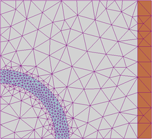
The main feature of the finite elements method is discreteization through the creation of a grid ( mesh ) composed of primitive ( finished elements ) coded shape (triangles and quadrilaterals for 2D domains, tetrahedrians and exhausts for 3D domains). On each elementary element characterized by this elementary form, the solution of the problem is assumed to be expressed by the linear combination of functions called basic functions O form functions ( shape functions ). It should be noted that sometimes the function is approximate, and the exact values ​​of the function will not necessarily be those calculated in the points, but the values ​​that will provide the lower error on the whole solution.

The typical example is that which refers to polynomial functions, so that the overall solution of the problem is approximate with a polynomial function in pieces. The number of coefficients that identifies the solution on each element is therefore linked to the degree of the chosen polynomial. This, in turn, rules the accuracy of the numerical solution found.

In its original form, and still more widespread, the finite elements method is used to solve poggiant problems on linear constitutive laws. Typical problems of efforts – deformations in the elastic field, the spread of heat within a material body. Some more refined solutions allow to explore the behavior of materials even in the strongly non-linear field, assuming plastic or visco-plastic behaviors. Furthermore, problems are sometimes considered coupled , within which different complementary aspects can be resolved simultaneously attributable each on account to an F.E.M. analysis separate. In this sense, the geotechnical problem of the behavior of an ground (geomechanical area) in the presence of aquifer filtration (hydrogeological sphere) are typical.

The finite elements method is part of the class of Gallërkin’s method, whose starting point is the so -called weak formulation of a differential problem. This formulation, based on the concept of derivative in the sense of distributions, of Lebnesgian integral and weighted media (through appropriate functions called test functions), has the great value of requesting the solution of realistic regularity characteristics for (almost) all engineering problems And it is therefore very useful descriptive tool.
Gallërkin type methods are based on the idea of ​​approximating the solution of the problem written in a weak form by linear combination of elementary functions (Shape Functions). The coefficients of this linear combination (also called “degrees of freedom”) become the unknowns of the algebraic problem obtained from discreteization. The finished elements are distinguished by the choice of polynomial basic functions in pieces. Other Gallërkin type methods such as spectral methods use different basic functions.

Phases to get to the model [ change | Modifica Wikitesto ]

To get to the model, the final elements follow the fundamental phases, each of which involves the insertion of errors in the final solution:

• Modeling: This phase is present in all engineering studies: we move from the physical system to a mathematical model, which abstracts some aspects of interest of the physical system, focusing attention on few variables aggregated of interest and “filtering” the rest. For example, in the calculation of the flexant moment of a beam, interactions at the molecular level are not taken into consideration. The physical if complex system is divided into subsystems. In the case in question it is not necessary, or you can think that it is a part belonging to a more complex system, for example of a ship or airplane. The subsystem will then be divided into finished elements to which a mathematical model will be applied. Unlike the analytical discussion, it is sufficient that the chosen mathematical model is adequate to the simple geometries of the finished elements. The choice of a type of element in a software program is equivalent to an implicit choice of the mathematical model that is at the base. The error that can bring the use of a model must be evaluated with experimental tests, an operation generally expensive in time and resources.
• Discreteization: in a numerical simulation it is necessary to move from an infinite number of degrees of freedom (a condition of the “continuum”) to a finite number (situation of the grid). Discreteization, in space or in time, aims to obtain a discreet model characterized by a finite number of degrees of freedom. An error given by the discrepancy with the exact solution of the mathematical model is inserted. This error can be appropriately evaluated if there is a mathematical model suitable for the entire structure (therefore preferable to be used with respect to the fem analysis) and in the absence of numerical calculation errors, this can be considered true using electronic calculators.

Characteristics of the elements [ change | Modifica Wikitesto ]

Each element is characterized by:

• Dimensione: 1D, 2D, 3D.
• Nodes: precise points of the element that identify its geometry. The value of a field or gradient affecting the entire structure is associated on each knot of the element. In the case of mechanical elements, the field is that of binding reactions and movements ( displacements ).
• Degrees of freedom: the possible values ​​that the fields or gradient can take in the nodes, two adjacent knots have the same values.
• Forces on the nodes: external forces applied on the nodes or the effect of binding reactions. There is a relationship of duality between constraint forces and reactions. Said
  ${displaystyle mathbf {f} }$

  the vector of external forces on a knot and

  ${displaystyle mathbf {u} }$

  The DOF carrier (from the English “Degree of Freedom”, degrees of freedom), takes on linearity between

  ${displaystyle mathbf {f} }$

  It is

  ${displaystyle mathbf {u} }$

  :

${displaystyle mathbf {ku} = mathbf {f}}$

Where

${displaystyle mathbf {K} }$

takes the name of stiffness matrix ( stiffness matrix ). This relationship identifies the duality between external forces and movements. The climbing product

${displaystyle mathbf {f} cdot mathbf {u} }$

is associated with the value of the work done by the external forces. The terms force, reaction binding e stiffness matrix , are extended beyond the scope of the mechanical structures in which the fem analysis was born.

• Constitutive properties: the properties of the element and its behavior. Then an isotropic material will be defined with elastic linear behavior, defined as a Young module and a Poisson coefficient.
• Solution of a system of equations, even non -linear resolved numerically by the elaborator. A negligible numerical error is introduced in the case of linear systems such as the one in analysis.

Type of finished elements [ change | Modifica Wikitesto ]

All programs that use the finished elements method for structural analysis are equipped with a bookshelf of finished elements (in the linear elastic field but also in the elastic-plastic one) single-dimensional, two-dimensional and three-dimensional to facilitate the modeling of a real structure.

The most common are as follows.

• monodimensionali:
  • to stay O biella O truss : 2 knots straight element that has a stiffness only for translations and is therefore the aim of transmitting only axial forces. It is normally used for the modeling of reticular structures.
  • grasses O beam : 2 knots straight element capable of transferring the nodes to which stiffness is connected for all 6 degrees of freedom and therefore aimed at transmitting all the types of stresses (axial forces and taglants and flexible and torching moments). It is used for the modeling of intelated structures. Some programs also have the beam element on elastic soil at the Winkler for modeling of foundation beams on elastic soil.
  • mullah O boundary O spring : two -knot straight element equipped with axial and/or rotational stiffness used to model various types of elastic bond such as for example the movements imposed;
  • harsh O rigel : rectilinear element at 2 infinitely rigid knots used to model an infinitely rigid bond between two finished elements;
• two -dimensional:
  • slab O stress plane : Plan element at 3 or 4 knots for states of flat effort that has only two degrees of freedom for node corresponding to the translations on its plan (membranial rigidity) and therefore aimed at transmitting only the efforts along its plan. It does not transfer any stiffness for the other degrees of freedom. Used for the modeling of structures loaded on their same level;
  • plate : plan for 3 or 4 knots that has only three degrees of freedom for node corresponding to the translation perpendicular to its plan and rotations compared to the two axes lying in the plane (flexional rigidity), and therefore acting only the cutting effort and the 2 Flexive moments. It does not transfer any stiffness for the other degrees of freedom. Used for the modeling of bidimensional structures inflected. Some software also have the plate element on soil to the Winkler used for the modeling of the Foundation on the elastic soil foundation;
  • plaster O shell O shell : plain element at 3 or 4 nodes consisting of the overlapping of the plate and the slab element and which therefore is equipped with both flexional stiffness and membrane.
  • flat deformation O plane strain : plan for 3 or 4 knots for plain deformation states which has only two degrees of freedom for node corresponding to the translations on its plan. It does not transfer any stiffness for the other degrees of freedom. It is used for the modeling of structures in which the thickness is prevalent compared to the other dimensions and where it can be considered the deformation in the thickness and therefore the state of deformation is considered slow as in the analysis of the sections of conduct or support walls.
  • Assialsimmetric : plan for 3 or 4 knots that represents a sector of a radiant of a radial symmetry structure. This element is used to model solid structures obtained for rotation of which the radial symmetry is frightened to analyze only a sector of the structure of the amplitude of a radiant. Each knot has 2 degrees of freedom corresponding to the translations on its plan;
• three -dimensional:
  • brick O solid element : element from 4 to 27 knots that has only three degrees of freedom for node corresponding to the three translations. It does not transfer any stiffness for the other degrees of freedom. It is a finite element capable of modeling solid structural elements in which there is no negligible dimension compared to the others. This element is able to interpret a three -dimensional tensional state. Used, for example, to model the stratigraphy of the soil.

Indicate [ change | Modifica Wikitesto ]

The definition of the geometry of the model that idealizes the real structure is carried out by placing nodes, or nodal points, on the structure in correspondence with characteristic points.

In positioning the nodes on the structure, some considerations must be kept in mind:

• The number of nodes must be sufficient to describe the geometry of the structure. For example, in correspondence with the bright-pillar, direction changes, etc.
• The knots must also be positioned in the points and on the discontinuity lines. For example, where the characteristics of the materials change, the characteristics of the sections, etc.
• Nodes can be placed in unnecessary points for the geometric definition of the structure but of which you want to know the movements and the internal stresses
• If the software does not foresee it, nodes must be positioned in correspondence with points where concentrated loads or nodal masses are applied
• You have to put knots in all the points that are intended to bind
• In the case of two -dimensional structures (plates, slabs, etc.) the subdivision ( mesh ) in two -dimensional finished elements must be dense enough to grasp the variations of effort or movement in the important regions for the purposes of analysis.

Single -dimensional formulation for second order equations [ change | Modifica Wikitesto ]

A differential equation with partial derivatives is given in the form:

${displaystyle -{frac {partial }{partial x}}left(alpha left(xright)cdot {frac {partial u}{partial x}}right)+sigma left(xright)cdot uleft(xright)=fleft(xright)}$

restricted to the domain

${displaystyle left[a,bright]}$

and contour conditions:

${displaystyle uleft({vec {x}}right)={vec {u_{x}}}}$

Where

${displaystyle {vec {x}}}$

is a carrier containing the points of

${displaystyle partial left[a,bright]}$

It is

${Displaystyle {vec {u_ {x}}}}}$

is a carrier containing the values ​​taken by the function

${displaystyle u}$

in such points. Conditions expressed in this form are also called by Dirichlet. It is also possible to provide the value assumed by the derivative before the function as a side conditions, and in this case Neumann conditions are called.

The finite elements method provides for the multiplication of both members for a test function

${displaystyle vleft(xright)}$

:

${displaystyle -vleft(xright)cdot {frac {partial }{partial x}}left(alpha left(xright)cdot {frac {partial u}{partial x}}right)+vleft(xright)cdot sigma left(xright)cdot uleft(xright)=vleft(xright)cdot fleft(xright)(forall vleft(xright))}$

The integration of both members on the domain leads to:

${displaystyle int _{a}^{b}-vleft(xright)cdot {frac {partial }{partial x}}left(alpha left(xright)cdot {frac {partial u}{partial x}}right)dx+int _{a}^{b}vleft(xright)cdot sigma left(xright)cdot uleft(xright)dx=int _{a}^{b}vleft(xright)cdot fleft(xright)dx(forall vleft(xright))}$

By exploiting the integration by parts it is possible to expand the first term:

${displaystyle int _{a}^{b}{frac {partial v}{partial x}}cdot {frac {partial u}{partial x}}cdot alpha left(xright)dx-left[vleft(xright)cdot alpha left(xright)cdot {frac {partial u}{partial x}}right]_{a}^{b}+int _{a}^{b}vleft(xright)cdot sigma left(xright)cdot uleft(xright)dx=}$

${displaystyle =int _{a}^{b}vleft(xright)cdot fleft(xright)dx(forall vleft(xright))}$

Therefore:

${displaystyle int _{a}^{b}{frac {partial v}{partial x}}cdot {frac {partial u}{partial x}}cdot alpha left(xright)dx+int _{a}^{b}vleft(xright)cdot sigma left(xright)cdot uleft(xright)dx=}$

${displaystyle =int _{a}^{b}vleft(xright)cdot fleft(xright)dx+left[vleft(xright)cdot alpha left(xright)cdot {frac {partial u}{partial x}}right]_{a}^{b}(forall vleft(xright))}$

The approximation to the finished elements is an approximation of Gallërkin and is performed at this point by discrtreting the domain in space

${displaystyle V_{h}}$

who admits a base

${Displaystyle Phin _{j},$

which is generally made up of polynomes at times of unrelated degree.

The discreteization of the domain in the single -dimensional case is made dividing

${displaystyle left[a,bright]}$

in intervals

${displaystyle left[x_{j-1},x_{j}right]}$

child

${displaystyle a=x_{0}$

It is

${Displaystyle H_ {J} = x_ {J} -X_ {J-1}}$

Functions

${Displaystyle Phi _ {J}}$

are generally expressed in the form:

${displaystyle phi _{j}left(xright)=left{{begin{array}{lr}{frac {1}{h_{k}}}cdot x+1-{frac {1}{h_{k}}}cdot x_{j}&(x_{j}-h_{k}leq x$

The weak formulation therefore provides for the determination of

${Displaystyle u_ {h} in v_ {h}}$

such that equality is verified:

${displaystyle int _{a}^{b}{frac {partial phi _{j}}{partial x}}cdot {frac {partial u_{h}}{partial x}}cdot alpha left(xright)dx+int _{a}^{b}phi _{j}left(xright)cdot sigma left(xright)cdot u_{h}left(xright)dx=}$

${displaystyle =int _{a}^{b}phi _{j}left(xright)cdot fleft(xright)dx+left[phi _{j}left(xright)cdot alpha left(xright)cdot {frac {partial u_{h}}{partial x}}right]_{a}^{b}(forall j=1,dots ,m)}$

Given the membership of

${displaystyle u_{h}}$

to space with base

${displaystyle left{phi _{j},j=1,dots ,mright}}$

, can be written

${displaystyle u_{h}}$

come:

${displaystyle u_{h}=sum _{i=1}^{m}U_{i}cdot phi _{i}left(xright)}$

By replacing and collecting, it is obtained:

${displaystyle sum _{i=1}^{m}U_{i}left(int _{a}^{b}{frac {partial phi _{j}}{partial x}}cdot {frac {partial phi _{i}}{partial x}}cdot alpha left(xright)dx+int _{a}^{b}phi _{j}left(xright)cdot sigma left(xright)cdot phi _{i}left(xright)dxright)=}$

${displaystyle =int _{a}^{b}phi _{j}left(xright)cdot fleft(xright)dx+left[phi _{j}left(xright)cdot alpha left(xright)cdot {frac {partial u_{h}}{partial x}}right]_{a}^{b}(forall j=1,dots ,m)}$

This equality is expressed in matricial form such as:

${displaystyle left[{begin{array}{cccc}a_{11}&a_{12}&…&a_{1m}\a_{21}&a_{22}&…&a_{2m}\…&…&…&…\a_{m1}&a_{m2}&…&a_{mm}end{array}}right]cdot left[{begin{array}{c}U_{1}\U_{2}\…\U_{m}end{array}}right]=left[{begin{array}{c}f_{1}\f_{2}\…\f_{m}end{array}}right]}$

where the terms of the matrices express themselves as:

${displaystyle a_{ij}=int _{a}^{b}{frac {partial phi _{j}}{partial x}}cdot {frac {partial phi _{i}}{partial x}}cdot alpha left(xright)dx+int _{a}^{b}phi _{j}left(xright)cdot sigma left(xright)cdot phi _{i}left(xright)dx}$

${displaystyle f_{j}=int _{a}^{b}phi _{j}left(xright)cdot fleft(xright)dx+left[phi _{j}left(xright)cdot alpha left(xright)cdot {frac {partial u_{h}}{partial x}}right]_{a}^{b}}$

The resolution of the linear system allows the determination of the coefficients

${Displaystyle u_ {i}}$

. These coefficients allow the determination of the approximation in the discreteized space located in the requested domain.

Case of constant coefficients and approximation to the center of gravity [ change | Modifica Wikitesto ]

In general, the determination of stiffness and load matrices requires the use of quadrature methods for calculating the value of the integrals defined. Special and interesting case, however, is the one in which the coefficients of the differential equation are all constant. In this case, an exact and particularly efficient resolution of the differential equation is possible. Assuming in fact:

${displaystyle left{{begin{array}{l}alpha left(xright)=alpha \sigma left(xright)=sigma \fleft(xright)=fend{array}}right.}$

The integrals that make up the elements of the matrices become:

${displaystyle a_{ij}=alpha int _{a}^{b}{frac {partial phi _{i}}{partial x}}cdot {frac {partial phi _{j}}{partial x}}dx+sigma int _{a}^{b}phi _{i}left(xright)cdot phi _{j}left(xright)dxqquad f_{i}=fcdot int _{a}^{b}phi left(xright)dx+alpha cdot left[phi _{j}left(xright)cdot {frac {partial u_{h}}{partial x}}right]_{a}^{b}}$

By replacing the form functions, the correct value is possible to find an exact formulation of the integral as a function of variables chosen. Considering a single element

${displaystyle k}$

constituting the domain, between the nodes I e

${displaystyle j=i+1}$

, with the definitions previously given of the functions

${displaystyle phi }$

A 2×2 type square stiffness matrix is ​​obtained:

${displaystyle {begin{aligned}A_{k}=left{a_{ij}right}_{i,j=k}^{k+1}&=left{alpha int _{x_{i}}^{x_{j}}{frac {partial phi _{i}}{partial x}}cdot {frac {partial phi _{j}}{partial x}}dx+sigma int _{x_{i}}^{x_{j}}phi _{i}left(xright)cdot phi _{j}left(xright)dxright}_{i,j=k}^{k+1}\&=left{alpha int _{x_{i}}^{x_{j}}{frac {1}{h_{k}}}cdot {frac {1}{h_{k}}}dx+sigma int _{x_{i}}^{x_{j}}left(1+{frac {1}{h_{k}}}cdot left(x-x_{i}right)right)cdot left(1+{frac {1}{h_{k}}}cdot left(x-x_{j}right)right)dxright}_{i,j=k}^{k+1}\&={frac {alpha }{h_{k}}}cdot left[{begin{array}{cc}1&-1\-1&1end{array}}right]+{frac {sigma h_{k}}{6}}cdot left[{begin{array}{cc}2&1\1&2end{array}}right]\end{aligned}}}$

Such matrices are the unique non -nil, given the form of the function

${displaystyle phi }$

. They go to constitute the stiffness matrix

${displaystyle A}$

, which is therefore modular starting from the matrices

${displaystyle A_{k}}$

defined above.

The same procedure can be implemented for the load matrix obtaining:

${displaystyle F_{k}={frac {fh_{k}}{2}}cdot left[{begin{array}{c}1\1end{array}}right]+left[{begin{array}{c}alpha cdot left[phi _{j}left(xright)cdot {frac {partial u_{h}}{partial x}}right]_{a}^{b}\alpha cdot left[phi _{j}left(xright)cdot {frac {partial u_{h}}{partial x}}right]_{a}^{b}end{array}}right]}$

By composing the matrices of the elements in the correct way you reach the final form of the linear system:

${displaystyle left[{begin{array}{ccccc}{frac {alpha }{h_{1}}}+{frac {2sigma h_{1}}{6}}&-{frac {alpha }{h_{1}}}+{frac {sigma h_{1}}{6}}&0&…&…\-{frac {alpha }{h_{1}}}+{frac {sigma h_{1}}{6}}&left({frac {alpha }{h_{1}}}+{frac {2sigma h_{1}}{6}}right)+left({frac {sigma }{h_{2}}}+{frac {2sigma h_{2}}{6}}right)&-{frac {alpha }{h_{2}}}+{frac {sigma h_{2}}{6}}&0&…\0&-{frac {alpha }{h_{2}}}+{frac {sigma h_{2}}{6}}&…&…&…\…&0&…&…&…\…&…&…&…&…end{array}}right]cdot left[{begin{array}{c}U_{1}\U_{2}\…\…\U_{m}end{array}}right]=left[{begin{array}{c}{frac {fh_{1}}{2}}+alpha cdot left[phi _{j}left(xright)cdot {frac {partial u_{h}}{partial x}}right]_{a}^{b}\{frac {fh_{1}}{2}}+{frac {fh_{2}}{2}}+2cdot alpha cdot left[phi _{j}left(xright)cdot {frac {partial u_{h}}{partial x}}right]_{a}^{b}\…\{frac {fh_{m}}{2}}+alpha cdot left[phi _{j}left(xright)cdot {frac {partial u_{h}}{partial x}}right]_{a}^{b}end{array}}right]}$

This simple solution is possible only in the case of constant coefficients, as mentioned above. In the case of non -constant coefficients, it is possible to settle for a very approximate but computationally simple and quick solution by carrying out an approximation to the center of gravity of the functions, that is, considering an average of the value of the functions at the extremes of each element:

${displaystyle left{{begin{array}{l}alpha ={frac {alpha left(x_{i}right)+alpha left(x_{j}right)}{2}}\sigma ={frac {sigma left(x_{i}right)+sigma left(x_{j}right)}{2}}\f={frac {fleft(x_{i}right)+fleft(x_{j}right)}{2}}end{array}}right.}$

This approximation allows you to exploit the results just achieved even in the case of non -constant coefficients, at the price of less precision.

Single -dimensional example [ change | Modifica Wikitesto ]

A typical problem, sometimes called the problem of Poisson’s equation, can be to find the function

${displaystyle u}$

whose laplacian is equal to a function

${displaystyle f}$

date. Poisson’s equation in a single -dimensional space is written as follows:

${displaystyle -u”(x)=f(x)}$

with various types of conditions at the edge, including for example:

${Displaystyle in (0) = u (1) = 0}$

${displaystyle u(0)=0qquad u'(1)=q}$

${Displaystyle u ‘(0) = u’ (1) = 0}$

${Displaystyle u ‘(0)+u (0) = 0qquad u’ (1)+u (1) = 0}$

The conditions in the outline in general can be divided into three groups:

• Conditions of Dirichlet: condition on function (order 0).
• Neumann conditions: derivative set condition before function with respect to the normal outgoing to the outline (order 1).
• Robin’s conditions: condition imposed on the linear combination of the value of the function and its derivative (mixed condition).

For example, if reference is made to the conditions of Dirichlet:

${Displaystyle in (0) = u (1) = 0}$

The variational form of the problem becomes to find

${displaystyle u}$

belonging to an appropriate functional space of functions that cancel to the edge that for each function

${displaystyle v}$

In the same functional space we have:

${displaystyle int limits _{0}^{1}u^{prime }v^{prime }dx=int limits _{0}^{1}fvdx}$

The approximation of the method to the elements is obtained by introducing a subdivision of the interval

${Displaystyle (0.1)}$

In under-intervals on each of which the solution will be taken to be polynomial. This allows you to write the approximate solution, indicated as

${displaystyle u_{h}}$

, by means of linear combination of the basic functions of the space of polynomial functions in pieces, indicated as

${displaystyle varphi _ {I}}$

:

${displaystyle u_ {h} = sum limits _ {j = 1}^{n} u_ {j} varphi _ _ _ _$

The coefficients

${Displaystyle u_ {j}}$

They are the unknowns of the discreet problem. Using how test functions the basic functions, in fact you get a set of n Equations:

${displaystyle sum limits _{j=1}^{n}U_{j}int limits _{0}^{1}varphi _{j}^{prime }varphi _{i}^{prime }dx=int limits _{0}^{1}fvarphi _{i}dxqquad (i=1,ldots ,n)}$

Indicating with

${displaystyle A}$

to the matrix:

${displaystyle A=[a_{ij}]=int limits _{0}^{1}varphi _{j}^{prime }varphi _{i}^{prime }dx}$

child

${displaystyle mathbf {U} }$

the vector of elements

${Displaystyle u_ {j}}$

and with

${displaystyle mathbf {F} }$

The vector of elements:

${displaystyle F_{i}=int limits _{0}^{1}fvarphi _{i}dx}$

The algebral problem to be solved is given simply by the linear system:

${displaystyle Amathbf {U} =mathbf {F} }$

At the matrix

${displaystyle A}$

It is called “stiffness matrix”.

The method of finished differences (FDM, from English Finite Difference Method ) is an alternative method to approximate the solutions of differential equations to partial derivatives. The main differences between the two methods are:

• The most attractive feature of the finished elements is the ability to manage complex geometries with relative simplicity. The finite differences are, in their basic form, restricted to simple geometries management, such as rectangles and some non -complex alterations.
• The methodology of the finished elements is simpler implementation.
• There are several ways to consider the differences finished a particular case of the approach to the finished elements. For example, the formulation of the finished elements is identical to the formulation of the differences for Poisson’s equation if the problem is discreetized using a rectangular form with each rectangle divided into two triangles.
• The quality of the approximation of the finished elements is greater than the corresponding approach to finished differences.

In general, the finite elements method is the method of choice for all types of analysis for structural mechanics (for example to calculate the deformation and tension of rigid bodies or the dynamics of the structures). In computational fluidodinamics, however, we tend to use other methods such as the finished volume method. Computational fluidodynamics problems require the discreteization of the problem in a large number of cells or nodes (in order of millions), therefore the cost of the solution favors simpler and minor approximations for each cell. This is particularly true for aerodynamic problems for planes and cars or for meteorological simulations.

Gallërkin’s method consists in the use of the same form functions used in the approximation within the above under-intervals, as weighing in the calculation of the residue to the minimum squares applied to the weak formulation of the structural problem.

• ( IN G. Alarish and A. Craig: Numerical Analysis and Optimization: An Introduction to Mathematical Modelling and Numerical Simulation
• ( IN ) K. J. Bathe: Numerical methods in finite element analysis , Prentice-Hall (1976).
• ( IN ) J. Chaskalovic, Finite Elements Methods for Engineering Sciences , Springer Verlag, (2008).
• ( IN ) O. C. Zienkiewicz, R. L. Taylor, J. Z. Zhu: The Finite Element Method: Its Basis and Fundamentals , Butterworth-Heinemann, (2005).

• ( IN ) Finite elements method . are British encyclopedia Encyclopaedia Britannica, Inc.
• FEM analysis – virtual community for simulation and numerical modeling . are It.Groups.yahoo.com . URL consulted on May 3, 2019 (archived by URL Original February 17, 2013) .
• Italian section of the Nafems “The International Association for the Engineering Analysis Community” . are nafems.it .
• TCN Consortium: Technologies for numerical calculation – Superior Training Center . are Consorzioopn.it .
• CISM – International Centre for Mechanical Sciences , Udine . are cism.it .
• What is fea (Method of finished elements) . are Knol.google.com . URL consulted on May 3, 2019 (archived by URL Original January 11, 2012) .
• The method of finished elements . are Calcolosture.net .