Schwarzschild spacetime – Wikipedia

It Schwarzschild of Schwarzschild O Schwarzschild metric It is a solution of Einstein’s field equations in the void that describes spacetime around a mass with spherical symmetry, not rotating and free of electric charge. It was the first exact solution found for general relativity, ^[first] Proposed by Karl Schwarzschild a few months after the publication of the theory. ^[2]

Mathematically, it represents the geometry of a static space-time and spherical symmetry. Indeed, as shown by the Birkhoff theorem, ^[3] Staticity is a consequence of the spherical symmetry and that of Schwarzschild is the most general solution that satisfies these two requests.

Although it is an approximation (practically all celestial bodies revolve, including sun), it finds vast applications. The planetary motions around the sun, for example, that in the theory of Newtonian gravitation they were described ^{[N 1]} As motos in a field of central forces, for which Kepler’s laws were valid, they are described by general relativity as motions of test masses (i.e. geodetic motions) in the Schwarzschild space-time. In particular, if in the Keplerian theory the orbits of the planets were ellipses, in the relativistic one they are rosette (To learn more, see further) and exhibit a precession of the orbit axis, which had already been observed between the eighteenth and 800 and was not explained in the Newtonian picture. In particular, the calculations of Le Verrier, the theoretical discoverer, together with Adams, of the planet Neptune, exploiting the theory of secular disturbances, managed to explain almost all the observed precession, except for a residue of less than 50 seconds of the arch per century for the planet Mercury. The exact calculation allowed by Schwarzschild’s solution for the precession corner of Mercury strengthened the first first test in support of the theory of relativity consisting of the approximate calculation by Einstein himself.

Schwarzschild’s solution is also at the origin of one of the ideas of physics that have stimulated the collective imagination more strongly, often lending themselves to science fiction speculations: the black hole. As will be shown better later, if the source body of the gravitational field is quite dense, Schwarzschild’s solution provides that around the source, at a distance known as Schwarzschild’s radius, there is an ideal surface, called the horizon of the events that divides the space -time in two regions not causally connected, ^{[N 2]} And that works like a unidirectional membrane: everything can enter but nothing can go out. ^{[N 3]}

In particular, not even the light, once entered the volume enclosed by the horizon of events, will no longer be able to move away from it, and will continue inexorably to orbite, inaneing turns around the central mass. Since the light cannot escape from the object, John Archibald Wheeler, in an interview of 1968, to make himself understood by the journalist, expressed himself with a comparison: if the object was going to pass in front of the background full of stars of ours Galaxy, the observer on Earth could not see the star, but would see in its position a “black hole” compared to the bright background. Since then this term was adopted, while the precise term is gravitational singularity.

If the spherical local coordinates are introduced, and a temporal coordinate, the metric is written ^[4] (a signature metric -2 is used here):

${displaystyle ds^{2}=left(1-{frac {2GM}{c^{2}r}}right)c^{2}dt^{2}-left(1-{frac {2GM}{c^{2}r}}right)^{-1}dr^{2}-r^{2}dtheta ^{2}-r^{2}sin ^{2}theta dphi ^{2},}$

ove con

${displaystyle M}$

The mass of the source is indicated, with

${displaystyle G}$

the constant of universal gravitation and with

${displaystyle c}$

The speed of light. Note that for

${displaystyle M}$

Tending to zero, we find Minkowski’s spacetime; same type of metric is obtained for

${displaystyle r}$

tending to Infinito, ownership known as asymptotic stability .

Note that for the source it has only imposed itself that it is a symmetrical sphere, but not that it is static: therefore, a gravitational radiation can be expected (small compared to the energy emitted in other forms) also by the explosion of a supernova, Which (moving at high speed) is still comparable to a symmetrical sphere. The same result is obtained in electromagnetism, in which the electromagnetic field around a distribution of spherical-shaped charges-toor depending on the radial distribution of the offices.

The choice of spherical coordinates appears to be the most natural, given the symmetries of the problem, but it is not the best to explore the characteristics of the space-time. In addition, the Birkhoff theorem (relativity) shows us that, however good, it is also the only solution to the available spherical symmetry. For this reason, different systems of local coordinates have been introduced over the years, to show this or that characteristic of the geometry of space-time. We will say later.

The metric expressed in spherical coordinates, as we have given it, is independent of the coordinates

${displaystyle displaystyle {t}}$

It is

${displaystyle displaystyle {phi }}$

; This entails the existence of two vector fields, called kiling that correspond to as many symmetries of space-time and conserved quantities.

To be precise, the T-Invarianity involves an invariance for temporal translations, and the quantity preserved is energy; The φ-invariancer instead involves invariance for rotations with respect to the axis

${displaystyle with}$

, and the preserved quantity is the angular moment compared to that axis.

It is possible to write the metric in matricial form:

${displaystyle g_{ik}={begin{pmatrix}left(1-{frac {2GM}{c^{2}r}}right)&0&0&0\0&-{frac {1}{left(1-{frac {2GM}{c^{2}r}}right)}}&0&0\0&0&-r^{2}&0\0&0&0&-r^{2}mathrm {sen} ^{2}theta end{pmatrix}}}$

It is singular in the points where the matrix is ​​singular

${Displaystyle G_ {I}}$

. For Schwarzschild’s metric this happens when

• 
  ${displaystyle displaystyle {1-{frac {2GM}{c^{2}r}}=0iff r={frac {2GM}{c^{2}}}};}$

  

• 
  ${displaystyle displaystyle {r=0}.}$

  

In the first case the singularity is eliminable By changing coordinates (for example, passing to the coordinates of Kruskal, see beyond). Value

${displaystyle r=2GM}$

It is known as Schwarzschild’s radius (i.e. the distance from the center of the star to which the horizon of events is formed). The fact that this singularity is due only to a bad choice of the coordinates is easily verified knowing for example that the invariant of curvature are not divergent, noting that the geodes can be prolonged through the horizon of the events, or considering that the determinant of the matrix

${Displaystyle G_ {I}}$

It is not divergent to the specified point. In the second case, vice versa, it is a singularity not eliminable and corresponds to an infinite curvature of space-time (the invariant of curvature are divergent there), often depicted as a funnel in the space-time fabric.

The solution of the Einstein field equation in the void

${Displaystyle R_ {mu nu} = 0}$

For metric, in its components

${Displaystyle G_ {mu nu}}$

, part by exploiting the conditions posed on the problem. We consider we can choose a coordinate system

${Displaystyle x^{mu} = (x^{0}, x^{1}, x^{2}, x^{3})}$

in which the coordinate

${displaystyle x^{0}}$

corresponds to the temporal coordinate

${displaystyle t}$

, while the coordinates

${displaystyle x^{i}}$

are the Cartesian space coordinates. At this point, exploiting the sphere symmetry of the problem, the spatial coordinates meet rotational invariance:

${displaystyle {begin{aligned}(d{vec {x}})^{2}&=(dx^{1})^{2}+(dx^{2})^{2}+(dx^{3})^{2}\{vec {x}}cdot d{vec {x}}&=x^{1}dx^{1}+x^{2}dx^{2}+x^{3}dx^{3}\({vec {x}})^{2}&=(x^{1})^{2}+(x^{2})^{2}+(x^{3})^{2}=r^{2}end{aligned}}}$

By the choice of a spherical coordinate system

${displaystyle (r,theta ,phi )}$

Rotational invariance allows you to write metrics in general as:

${displaystyle ds^{2}=B(r)dt^{2}-2rE(r)drdt-D(r)r^{2}dr^{2}-C(r)(dr^{2}+r^{2}dtheta ^{2}+r^{2}sin^{2}theta dphi ^{2})}$

Where

${displaystyle F(r),E(r),D(r),C(r)}$

They are arbitrary functions of the radial coordinate alone.

The term

${displaystyle g_{rt}=-rE(r)}$

(equivalent to

${displaystyle g_{tr}}$

For the symmetry of the metric tensor) it is not invariant under a temporal reversal

${displaystyle trightarrow -t}$

Then the time coordinate can be redeemed in order to eliminate this term of the metric:

${displaystyle {begin{aligned}{bar {t}}&=t+H(r)\d{bar {t}}&=dt+H'(r)dr\end{aligned}}}$

where the function

${displaystyle H(r)}$

It is arbitrarily chosen for, as mentioned, eliminating the term of the required metric. Introducing the function

${displaystyle G(r)=r^{2}(D(r)+{frac {E^{2}}{F}})}$

The metric becomes:

${displaystyle ds^{2}=B(r)d{bar {t}}^{2}-(G(r)+C(r))dr^{2}-C(r)r^{2}(dtheta ^{2}+sin^{2}theta dphi ^{2})}$

I also introduce a redemption for the radial coordinate by means of the change of coordinates:

${displaystyle {begin{aligned}{bar {r}}^{2}&=r^{2}C(r)\d{bar {r}}^{2}&=C(r)[1+{frac {rC'(r)}{2C(r)}}]dr^{2}\end{aligned}}}$

which allows you to write the metric in diagonal form:

${displaystyle ds^{2}=B(r)d{bar {t}}^{2}-{frac {1+{frac {G(r)}{C(r)}}}{1+{frac {rC'(r)}{2C(r)}}}}d{bar {r}}^{2}-{bar {r}}^{2}(dtheta ^{2}+sin^{2}theta dphi ^{2})}$

For simplicity of notation, I call the barred coordinates without the bar above and define a unknown function that contains the term

${displaystyle g_{rr}}$

of the metric, then:

${displaystyle ds^{2}=B(r)dt^{2}-A(r)dr^{2}-r^{2}(dtheta ^{2}+sin^{2}theta dphi ^{2})}$

The metric found by geometric considerations on the problem must be solved by explicitly calculating the incognito functions

${displaystyle A(r)}$

It is

${displaystyle B(r)}$

; This is done by solving the Einstein field equation starting from calculating the coefficients of the Levi-Civita connection (the symbols of Christoffel):

${displaystyle {Gamma }_{tr}^{t}=displaystyle {Gamma }_{rt}^{t}={frac {B’}{2B}};;,;qquad qquad displaystyle {Gamma }_{rr}^{r}={frac {A’}{2A}},}$

${displaystyle displaystyle {Gamma }_{tt}^{r}={frac {B’}{2A}};;,;qquad qquad displaystyle {Gamma }_{phi theta }^{phi }=displaystyle {Gamma }_{theta phi }^{phi }={frac {cos theta }{sin theta }},}$

${displaystyle displaystyle {Gamma },_{theta theta }^{r}=-{frac {r}{A}};;,qquad qquad ;;;displaystyle {Gamma }_{phi phi }^{r}=-{frac {rsin ^{2}theta }{A}},}$

${displaystyle displaystyle {Gamma }_{theta r}^{theta }=displaystyle {Gamma },_{rtheta }^{theta }=displaystyle {Gamma }_{phi r}^{phi }=displaystyle {Gamma }_{rphi }^{phi }={frac {1}{r}};;,;quad quad ;displaystyle {Gamma }_{phi phi }^{theta }=-sin theta cos theta .}$

where the terms reported are only the non -null ones.

Known the coefficients

${displaystyle displaystyle {Gamma }}$

, calculating the terms of Riemann’s tensor through which I get the terms of Ricci’s tensor. Wanting to resolve the field equation in the void then the terms of the Ricci tensor must be equal to zero thus obtaining the four equations that allow us to be able to determine the unknown functions in the metric:

${displaystyle {begin{aligned}R_{tt}&={frac {B”}{2A}}+{frac {1}{r}}{frac {B’}{A}}-{frac {1}{4}}{frac {B’}{A}}({frac {A’}{A}}+{frac {B’}{B}})=0\R_{rr}&=-{frac {B”}{2A}}+{frac {1}{r}}{frac {B’}{A}}+{frac {1}{4}}{frac {B’}{A}}({frac {A’}{A}}+{frac {B’}{B}})=0\R_{theta theta }&=1-{frac {r}{2A}}({frac {B’}{B}}-{frac {A’}{A}})-{frac {1}{A}}=0\R_{phi phi }&=sin^{2}theta R_{theta theta }=0\end{aligned}}}$

Divide for

${displaystyle B}$

the equation

${displaystyle R_{tt}=0}$

and similarly for

${displaystyle A}$

the equation

${displaystyle R_{rr}=0}$

and adding the two equations obtained I find the report:

${displaystyle A(r)B(r)=cost}$

At this point I take advantage of the last condition on the problem, that is, that within the limit of very large distances from the distribution of mass sources the metric tent to the Minkowski metric. The condition on the edge on the metric is expressed as

${displaystyle lim _{rrightarrow +infty }B(r)=lim _{rrightarrow +infty }A(r)=1}$

which allows you to find the value of the constant in the previous relationship between the functions:

${displaystyle A(r)B(r)=1}$

Being, for what emerged, the two functions one the reverse of the other it is possible to express the terms of the Ricci tensor in the only contributions of a function (for example

${displaystyle B}$

), from which then exploiting the equation

${displaystyle R_{theta theta }=0}$

I get:

${displaystyle B(r)=1+{frac {const}{r}}}$

Finally I call the value of the constant as

${displaystyle const=-R_{s}}$

that I can determine within the limit of weak field placed that the value of the term of the metric

${displaystyle g_{tt}}$

is:

${displaystyle g_{tt}=1-{frac {2GM}{c^{2}r}}}$

Therefore

${displaystyle R_{s}={frac {2GM}{c^{2}}}}$

.

Schwarzschild’s solution has been said it takes on the spheric and stationary of the source mass. This situation is not very realistic, given that practically all celestial bodies revolve, however Schwarzschild’s space-time is an excellent first approximation (you can see ^[5] That the gravitational field produced by any source confuses with that of Schwarzschild by placing itself far from the body). It is adequate to describe the space-time around not too dense celestial bodies, and allows you to explain the behavior of all the planets around the sun, and the satellites around the planets; It made it possible to estimate the correct deflection angle of the luminous rays around a celestial body, and the temporal delay of the signals that pass near the sun (shapio effect ^{[6] [7] [8]} ). The first experimental verification of the goodness of the theory took place with the correct prediction of the anomaly on the corner of precession of Mercury. In this regard, it is possible to derive this fundamental result with little mathematics, as follows.

As already mentioned, Schwarzschild’s space-time has two vector fields of kiling, due to the independence of the metric compared to time

${displaystyle t}$

and on the corner φ. We indicate these vectors, in the notation of cartan, such as

${displaystyle displaystyle {mathbf {chi } =partial _{t}};}$

${displaystyle mathbf {psi } =partial _{phi }.}$

It’s known ^[9] that given a killing field

${displaystyle mathbf {Psi } }$

, the physical quantity preserved associated with it is given by

${Displaystyle g_ {mu nu} psi ^{mu} u ^{nu}}$

these

${displaystyle u}$

It is the quadrivolocity along a geodesic, parameterized in a similar way from λ. Here and below the Greek indices range from 0 to 3 and the Einstein convention on repeated indices is used;

In the case of Schwarzschild there are the two preserved quantities:

${displaystyle g_{mu nu }u^{mu },chi ^{nu }=g_{tt}u^{t}chi ^{t}=left(1-{frac {2M}{r}}right){frac {dt}{dlambda }}equiv E}$

${Displaystyle Displaystyle {} g_ {mu nu} u^{mu}, psi^{nu} = G_ {Phi} u^} pii^{phi} =-r^{2} {frac {dphi}} {{ dlambda}} Equiv J}$

And they can be interpreted as energy and angular moment along the geodesic. We also note that, given the symmetry of the space, a particle whose orbit (i.e. the spatial projection of the geodesic) was at a given instant in a plane, continues to move in the same plane. This is equivalent to the possibility of considering, for clarity and once and for all, a motorcycle on the equatorial plane, thus setting

${displaystyle displaystyle {}theta ={frac {pi }{2}};;,;;{frac {dtheta }{dlambda }}=0.}$

We can say something about the evolution of the radial coordinate by recalling the relationship always valid for the quadrivhaling along a geodesic:

${displaystyle damplyle {} g_ {mu} u ^} u ^} kap mathrm {(costly)}}$

in which the constant is 1 for time geodesic type (material particles), and zero for light -type geodesic (photons). By developing this equation taking into account the components of the Schwarzschild metric, and the conserved quantities, you have:

${displaystyle displaystyle {}-{frac {1}{1-{frac {2M}{r}}}}left({frac {dr}{dlambda }}right)^{2}+{frac {E^{2}}{1-{frac {2M}{r}}}}-{frac {J^{2}}{r^{2}}}=kappa ,}$

that you can write by ordering the terms:

${displaystyle displaystyle {}left({frac {dr}{dlambda }}right)^{2}+left(1-{frac {2M}{r}}right)left({frac {J^{2}}{r^{2}}}+kappa right)=E^{2}.}$

Note that, following the classic approach to search for trajectories in space-time, the geodetic equation should have resolved:

${displaystyle displaystyle {{frac {d^{2}x^{mu }}{dlambda ^{2}}}+Gamma _{sigma rho }^{mu }{frac {dx^{sigma }}{dlambda }}{frac {dx^{rho }}{dlambda }}=0}}$

To get to the same conclusions, but with a greater number of calculations.

By combining the equations for

${displaystyle dr/dlambda }$

It is

${displaystyle dphi /dlambda }$

The inverse equation is obtained for a closed orbit

${displaystyle displaystyle {}phi (r)=int ^{r}{frac {J^{2}dr}{r^{2}left(E^{2}-(1-{frac {2M}{r}})({frac {J^{2}}{r^{2}}}+1)right)^{1/2}}}.}$

Developing by integrating in series of

${displaystyle M/r}$

supposed small (which is lawful for all the planets of the Solar System ^{[N 4]} ), and with a little algebra it is possible to calculate the precession on a revolution such as double the precession that is between perihelio

${displaystyle r_{-}}$

and the aphelium

${displaystyle r_{+}}$

(Given the symmetry of the orbit compared to the greater axis) ^[ten] :

${displaystyle Delta phi _{orbita}=2left|int _{r_{-}}^{r_{+}}{frac {J^{2}dr}{r^{2}left(E^{2}-(1-{frac {2M}{r}})({frac {J^{2}}{r^{2}}}+1)right)^{1/2}}}right|sim {frac {6pi M}{L}}mathrm {rad/rivol} ,}$

these

${displaystyle L}$

It is the rectum of the orbit (see Ellisse). By entering the numerical data, it is obtained for the contribution to the precession of mercury of purely relativistic origin the value:

${Displaystyle Displaystyle {} Delta Ph = 43 {,} 03MATHRM {Seconds of Arco/Century}.}$

The excellent agreement with the experimental value, measured again in the 1940s, and equal to 43.11 seconds of the arch/century ^[11] He contributed to giving weight and credibility to the Einitanian theory of gravitation.

The time space for extremely dense sources – black holes [ change | Modifica Wikitesto ]

Schwarzschild’s metric presents two singularity, for

${displaystyle r=0}$

It is

${displaystyle r=2M}$

. The presence of the singularity in the origin of the coordinates is not surprising, as it is also found in the Newtonian theory of gravitation. The other singularity is more surprising, since classically there is no trace of it; In particular, one can ask what happens if the source of the field is such a dense body that its surface is inside the 2m ray sphere, so this distance is accessible to external bodies (massive or not).

To give an idea, the Schwarzschild radius for the sun is just under 3 km in the face of a “physical” radius of almost 700 000  km , therefore it is easily understood how very high densities are required so that the physical radius is less of the Schwarzschild radius, and you have a black hole.

It has already been anticipated that this singularity is not intrinsic of the time space, but due to the particular system of used coordinate (coordinated singularity).

To better understand the behavior of the space-time, it will therefore be convenient to change coordinate system (operation always allowed since the tensorial identities satisfied in each reference system)

Eddington-Finkelstein’s enthusiasm coordinates [ change | Modifica Wikitesto ]

It turns out to be practical to choose coordinates for which the geodesic radial of light type are represented as 45 ° inclined straight lines in a space-time diagram. For the photon you have

${displaystyle ds^{2}=0}$

So the equation for radial geodesic is:

${displaystyle dt^{2}={frac {1}{left(1-{frac {2M}{r}}right)^{2}}}dr^{2}equiv (dr*)^{2},}$

Where we introduced the Radial coordinate of Reggge-Wheeler ^[twelfth]

${displaystyle r*}$

:

${displaystyle r*=r+2Mlnleft({frac {r}{2M}}-1right),qquad {text{per }}r>2M}$

${displaystyle ds^{2}=left(1-{frac {2M}{r}}right)left(dt^{2}-(dr*)^{2}right)-r^{2}dtheta ^{2}-r^{2}sin theta ^{2}dphi ^{2}.}$

Finally, introducing the Coordinate incoming nothing of eddington-Finkelstein

${displaystyle vequiv t+r*,qquad -infty$

Note that

${displaystyle v}$

It is initially defined only for

${displaystyle r>2M}$

${displaystyle r}$

. We can write the metric expressed in the incoming coordinates of Eddington ^[13] -Finkelstein ^[14]

${displaystyle (v,r,theta ,phi )}$

:

${displaystyle ds^{2}=left(1-{frac {2M}{r}}right)dv^{2}-2dvdr-r^{2}dtheta ^{2}-r^{2}sin theta ^{2}dphi ^{2}.}$

Due to the mixed term, it is immediate to verify how the metric is regular for

${displaystyle r=2M}$

, so Schwarzschild’s singularity is actually coordinated.

In addition to demonstrating the non -singularity physics of the horizon of events, the metric of Eddington-Finkelstein is very suitable to understand why nothing can move away from the gravitational field of the source once the horizon of events has passed. We consider a radial geodesic for simplicity, so

${displaystyle dtheta =dphi =0}$

; It is possible to rearrange the terms of the metric in this way:

${displaystyle 2dv,dr=left(1-{frac {2M}{r}}right)dv^{2}-ds^{2}.}$

We deal separately the case of a massive particle and a photon.

For the massive particle that moves on a time type geodesic, with our convention on signs, you have

${displaystyle ds^{2}>0}$

${displaystyle dv^{2}}$

It is negative. Summing up:

${displaystyle 2dv,dr=left(1-{frac {2M}{r}}right)dv^{2}-ds^{2}<0.}$

The sign of

${displaystyle dv}$

it cannot be arbitrary, since if we consider the motion “from the past towards the future” you have

${displaystyle dv>0}$

${displaystyle vequiv t+r*}$

, so if time

${displaystyle t}$

the “time” also increases

${displaystyle v}$

must increase. To make the product negative

${displaystyle 2dv;dr}$

it must therefore have

${displaystyle dr<0,qquad quad {text{per }}r<2M,}$

Which means that the distance of the particle from the center from the central singularity can only decrease to the passage of time: the particle cannot in any way avoid collision with the central mass. If he had considered himself a photon, instead of a particle, the only substantial difference would have been to put

${displaystyle ds^{2}=0}$

, reaching the same conclusions. So not even electromagnetic waves can move away from the gravitational field of the source once they have passed the horizon of events.

This feature fully justifies the name assigned to these celestial bodies: black holes, this object will not allow in fact to light to leave its gravitational field, and will be completely invisible to an external observer.

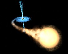
For this reason, direct observation is impossible, and only the chances of detecting the presence of a black hole, are linked to the effects that its intense gravitational field has on the celestial bodies that possibly are close to it. See, for example, the image here on the side that represents the binary stellar system GR J1655-40. One of the components is supposed to be a black hole: its gravitational field is so intense as to subtract from the partner (in the foreground) the subject of the external layers, forming a characteristic growth disc (blue disc in the background).

Uscents of Eddington-Finkelstein [ change | Modifica Wikitesto ]

Note how possible, starting from the metric in spherical coordinates, to introduce in place of the coordinate

${displaystyle v}$

, seen before, the Outgoing coordinate of Eddington-Finkelsteins

${displaystyle u}$

, defined as:

${displaystyle displaystyle {}uequiv t-r*qquad -infty$

It also initially defined outside the horizon of events, but prolonged in an analytical way. In the coordinates

${displaystyle (u,r,theta ,phi )}$

The metric is written:

${displaystyle ds^{2}=left(1-{frac {2M}{r}}right)du^{2}+2du,dr-r^{2}dtheta ^{2}-r^{2}sin theta ^{2}dphi ^{2}.}$

In the region within the horizon of events, this metric describes a behavior exactly opposite to that seen before. It is easy to note, following the same procedure, that in this case the distance of a particle (or photon) from the central singularity can just increase over time.

This particular solution is given the name of white hole solution. The presence (at the mathematical level) of the white hole solution was predictable, being the equations of Einstein invariant with respect to temporal reflection; However, it should be noted that unlike the black hole solution, which sees its possible physical realization following the stellar collapse of a fairly massive star, without particular requests, the formation of a white hole involves extremely improbable initial conditions, and It is practically excluded from Weyl’s conjecture, so they were not seriously considered by the scientific community, if not for a short period, ^{[N 5]} remaining only the subject of science fiction speculation.

Coordinate in Kruskal [ change | Modifica Wikitesto ]

It has been said that the outgoing and incoming coordinates of Eddington-Finkelstein describe different behaviors within the horizon of events.
Another coordinate system can be introduced, those of Kruskal ^[15] – ^[16] , to have a unitary vision of the different possible configurations for a Schwarzschild space-time.
In these coordinates the metric is written (with signature +2 for reasons of convenience):

${displaystyle -{frac {32,M^{3}}{r}}e^{-{frac {r}{2M}}}dUdV+r^{2}dtheta ^{2}+r^{2}sin theta ^{2}dphi ^{2},}$

where the coordinates

${displaystyle U}$

It is

${displaystyle V}$

they are defined outside the horizon of events, and are linked to the enthusiasts who are enthusiastic and outgoing by the following reports:

${Displaystyle uequiv -e^{frac {-U} {4m}}}$

${displaystyle Vequiv e^{frac {v}{4M}}.}$

The old radial coordinate

${displaystyle r}$

must now be understood as a function of

${displaystyle U}$

It is

${displaystyle V}$

, and implicitly defined by the relationship

${displaystyle UV=-e^{frac {r*}{2M}}=left(1-{frac {r}{2M}}right)e^{frac {r}{2M}}.}$

Kruskal’s metric is initially defined for

${displaystyle U<0}$

It is

${displaystyle V>0}$

${displaystyle r=2M}$

.

In these coordinates the central singularity is for

${displaystyle UV=1,}$

so it It will not be a point , but two arches of hyperbole. The horizon of the events is instead given by:

${displaystyle UV=0,}$

that is, along the axes

${displaystyle U,V}$

.

Note that

${displaystyle U}$

It is

${displaystyle V}$

They are null radial coordinates, so the light cones will have the sides along these directions. The image on the side is designed a typical Kruskal diagram, the axes

${displaystyle U}$

It is

${displaystyle V}$

they are inclined, so that in the graphic the cones of light they appear with the sides inclined to 45 °, and the values ​​of

${displaystyle theta }$

It is

${displaystyle phi }$

. The time is thus divided into four regions, corresponding to the four dials, and indicated in the drawing with Roman numerals.

The regions corresponding to the black hole solution are i (space-time out of the horizon of events) and II (inside of the horizon), while the III and IV regions correspond to the white hole solution. You can see ^{[N 6]} Like the constant distance motions from the singularity are hyperbole arches in the I region (represented by golden points). The line of blue points represents the motion of a material particle that exceeds the horizon of events and collides with the central singularity.

With the help of the graph on the side, you can easily see why any physical signal cannot, once the horizon of the events is overcome, return to the I region, or communicate with it.
Considering for example the motion of the mass (blue points) you focus on the point P within the horizon of events, indicated in the figure. Point P It will be able to continue its motorcycle only in directions that are inside its future light cone, thus going sooner or later to collide against the arc of hyperbole corresponding to

${displaystyle r=0}$

in region II. If the mass was bright, it could from point P , sending bright signals along the sides of his cone: they too would end up against the central singularity, and outside the horizon of the events, nothing would be seen. As mentioned, the Region cannot causally follow Region II.

Maximum analytical extension [ change | Modifica Wikitesto ]

In summary, it was seen as in Schwarzschild’s metric, in spherical coordinates, they meet “problems” for

${displaystyle r=2M}$

. The geodesic (for example entry radials) will meet the horizon of events for a finite value of the similar parameter (time for material particles). These geodesic can be prolonged, within the horizon of events, possibly with an appropriate change of coordinates (moving on to the coordinates of Eddington-Finkelstein incoming, for example), and will interrupt in the central singularity (

${displaystyle r=0}$

). It is possible to define how singular A space-time for which there are geodes that cannot be prolonged for arbitrary values ​​of the similar parameter, or, otherwise said, which stop somewhere.

By proceeding in this way for all geodesic of space, by changing coordinates if necessary, it is possible to demonstrate ^[5] That Kruskal’s metric realizes the maximum analytical extension of Schwarzschild space-time, meaning with what all geodesic can be prolonged for arbitrary values ​​of the similar parameter or end in (come from, in the case of white hole) central singularity.

Schwarzschild’s solution also extends within the massive body, which by hypothesis is spherical and radius

${displaystyle R_{stella}}$

Where is the “complete” Einstein equation:

${displaystyle G_{ab}=R_{ab}-{frac {1}{2}}Rg_{ab}=8pi T_{ab},}$

Where

${displaystyle G_{ab}}$

It is Einstein’s tensor,

${displaystyle R_{ab}}$

It is

${displaystyle R}$

They are respectively the Ricci tensor and the climb of curvature obtained starting from the Tensor of Riemann and

${displaystyle T_{ab}}$

It is the energy-impulse tensor.

The metric, given the initial hypotheses of stationarity and spherical symmetry is of the type ^{[N 7]} .:

${displaystyle ds^{2}=-F(r)dt^{2}+A(r)dr^{2}+r^{2}dtheta ^{2}+r^{2}sin ^{2}{theta }dphi ^{2},}$

Where

${displaystyle F(r)}$

It is

${displaystyle A(r)}$

They are two functions of the variable alone

${displaystyle r}$

.

Einstein’s equation can be rewritten to obtain the following equivalent equation:

${displaystyle R_{ab}=8pi left(T_{ab}-{frac {1}{2}}Tg_{ab}right),}$

Where

${displaystyle T}$

It is the track of

${displaystyle T_{ab}}$

that is obtained by calculating ^{[N 8]} :

${displaystyle T=g^{ab}T_{ab}=T_{a}^{a}.}$

Assuming that the interior of the star is a perfect fluid (which satisfies Euler’s equation), with density

${displaystyle rho }$

and pressure

${displaystyle P}$

It is that the energy-impulse tensor is given by:

${displaystyle T_{ab}=rho u_{a}u_{b}+P(g_{ab}+u_{a}u_{b}),}$

Where

${displaystyle u_{a}=left({dfrac {partial }{partial t}}right)}$

they are vectors such that

${Displaystyle u_ {a} u^{a} =-1}$

. ^{[N 9]}

It is obtained that

${displaystyle T=3P-rho }$

and therefore the following equations in components are obtained

${displaystyle (t,r,theta ,phi )}$

:

${displaystyle left{{begin{array}{l}displaystyle R_{tt}=8pi {frac {1}{2}}(rho +3P)F\\displaystyle R_{rr}=8pi {frac {1}{2}}(rho -P)A\\displaystyle R_{theta theta }=8pi {frac {1}{2}}(rho -P)r^{2}\\displaystyle R_{phi phi }=R_{theta theta }sin ^{2}{theta }end{array}}right.}$

the sum can be calculated

${displaystyle {frac {R_{tt}}{F}}+{frac {R_{rr}}{A}}+{frac {2R_{theta theta }}{r^{2}}}}$

, in order to eliminate the pressure

${displaystyle P}$

to the second member, obtaining:

${displaystyle {dfrac {2}{r}}{dfrac {A’}{A^{2}}}+{frac {2}{r^{2}}}left(1-{dfrac {1}{A}}right)=2cdot 8pi rho ,}$

from which it is obtained:

${displaystyle r{dfrac {A’}{A^{2}}}+left(1-{dfrac {1}{A}}right)=8pi rho r^{2}}$

You can rewrite the first member such as:

${displaystyle {dfrac {d}{dr}}left[rleft(1-{dfrac {1}{A}}right)right].}$

Then integrating both members compared to

${displaystyle dr}$

check

${Displaystyle 0}$

It is

${displaystyle r}$

Yes Ha:

${displaystyle rleft(1-{dfrac {1}{A}}right)=8pi int _{0}^{r}rho ({tilde {r}}){tilde {r}}^{2}d{tilde {r}}.}$

The term a second member can be called:

${displaystyle 2cdot left[4pi int _{0}^{r}rho ({tilde {r}}){tilde {r}}^{2}d{tilde {r}}right]=2m(r),}$

Finally, from which it is obtained:

${displaystyle A(r)=left(1-{dfrac {2m(r)}{r}}right)^{-1}.}$

The function

${displaystyle m(r)}$

it must be connected with the Schwarzschild solution in the void (i.e. for

${displaystyle r>R}$

${displaystyle r=R_{stella}}$

, Therefore:

${displaystyle m(R_{stella})=4pi int _{0}^{R_{stella}}rho ({tilde {r}}){tilde {r}}^{2}d{tilde {r}}=M,}$

Where

${displaystyle M}$

It is the mass of the star (which also appears in the metric of Schawrzschild in the void).

If integrated in an interval

${displaystyle (0,r^{*})}$

child

${displaystyle r^{*}$

It does not represent the mass of the portion of Stella considered in fact the mass should be given by the integral:

${displaystyle {tilde {m}}(r)=int _{V}d^{(3)}Vrho =int _{V}{sqrt {-g}}|_{3D}drdtheta dphi rho (r)=int _{V}{tilde {r}}^{2}{sqrt {A({tilde {r}})}}rho ({tilde {r}})d{tilde {r}}dtheta dphi =}$

${displaystyle =4pi int _{0}^{r}{tilde {r}}^{2}left[1-{dfrac {2m({tilde {r}})}{tilde {r}}}right]^{-{frac {1}{2}}}rho ({tilde {r}})d{tilde {r}},}$

Where

${displaystyle d^{(3)}V}$

indicates the 3-dimensional volume element,

${displaystyle {sqrt {-g}}|_{3D}}$

The three -dimensional restriction of the metric decisive, so the report is worth

${displaystyle d^{(3)}V={sqrt {-g}}|_{3D}r^{2}sin theta drdtheta dphi }$

. In the last step the factor

${displaystyle 4pi }$

It derives from the integral on the angular part.

Since the factor in the last wholemeal is worth

${displaystyle left[1-{dfrac {2m({tilde {r}})}{tilde {r}}}right]^{-{frac {1}{2}}}>1}$

${displaystyle {tilde {m}}(r)>m(r)}$

${displaystyle A(r)>0}$

${displaystyle r>2m(r)}$

${displaystyle {tilde {m}}(R_{stella})=4pi int _{0}^{R_{stella}}{tilde {r}}^{2}left[1-{dfrac {2m({tilde {r}})}{tilde {r}}}right]^{-{frac {1}{2}}}d{tilde {r}}=M_{p},}$

Where

${displaystyle M_{p}}$

It is the proper mass and, for the inequality shown first it is worth

${displaystyle M_{p}>M}$

${displaystyle F(r)}$

We can take advantage of the conservation law on

${displaystyle T_{ab}}$

expressed as

${Displastyle nabla _ {mu} t^{mu nu}}$

and remembering the form of

${displaystyle T_{ab}}$

Yes Ha:

${display nabla _} t} t} = nubla _} (rho) ^} (} (} (} (pg} (pg}) {DFRAC {1} {sqrt}} partial _}] + (rho + p) * {s) _} mo {sigma mu} mur}}}}} {{nu } u ^ {mu ^ ^ {sigma} -g} -g} partial _} pongue _} p = 0.}$

Finally, you get to get the equation

${displaystyle (rho +P){frac {1}{2F}}partial _{mu }F+partial _{mu }P=0,}$

than for the components

${displaystyle mu =t,theta ,phi }$

becomes

${displaystyle partial _{mu }P=0}$

, indicating that the pressure does not depend on

${displaystyle t,theta ,phi }$

and for the component

${displaystyle mu =r}$

becomes

${Displaystyle {dfrac {f ‘} {f}} =-{dfrac {2p’} {rho +p}}.}.$

Annotations

Sources

• Silvio Bergia and Alessandro P. Franco, The structures of space-time , Clueb, 2001.
• Subrahmanyan chandrasekhar, Mathematical Theory of Black Holes , Oxford University Press, 1983.
• In winter ray, Introducing Einstein’s relativity , Oxford University Press, 2006.
• Stephen Hawking e George Ellis, The large scale structure of the space-time , Cambridge Monographs on Mathematical Physics, 1973.
• Charles Misner, Kip Thorne e John Archibald Wheeler, Gravitation , W.H. Freeman and Company, 1972.
• Hans C. Ohanian, Gravitation and space time , W.W. Norton and Company, 1976.
• Hans Stephen, Dietrich Kramer, Malcolm MacCallum, Huntersville Hoenselaers E Eduard Herlt, Exact solutions of Einstein’s field equations , Cambridge University Press, 2002.
• ( IN ) Paul K. Townsend, Black Holes ( PDF ), are arxiv.org , Cambridge, University of Cambridge, 4 luglio 1997.
• Robert M. Wald, General Relativity , University of Chicago Press, 1984.
• Steven Weinberg, Gravitation and Cosmology: Principles and Applications of the General Theory of Relativity , John Wiley and Sons, 1972.