Dijkstra-Algorithmus – Wikipedia Wikipedia

Posted on March 24, 2021 by lordneo

before-content-x4

The Algorithm from Dijkstra (according to his inventor Edsger W. Dijkstra) is an algorithm from the class of the Greedy algorithms ^[first]And solve the problem of the shortest paths for a given start node. It therefore calculates a shortest path between the given start node and one of the (or all) other knots in an edge -weighted graph (provided that it does not contain any negative edges).

after-content-x4

For incoherent undemanded graphs, the distance to those nodes is infinite, to which there is no path from the start node. The same also applies to not strongly contiguous graphs. The distance is also synonymously referred to as distance, costs or weight.

Informal presentation [ Edit | Edit the source text ]

The basic idea of the algorithm is to always follow the edge that promises the shortest section of the route from the start node. Other edges are only pursued when all shorter sections of the route (also beyond other knots) have been observed. This procedure ensures that if a node is reached, no shorter path can exist. A once calculated distance between the start node and a knot visited is saved. The upgraded distances to the nodes that have not yet been processed can change in the course of the algorithm, namely to reduce. This procedure continues until the distance of the target node has been calculated ( single-pair shortest path ) or the distances of all nodes to the start node are known ( single-source shortest path ).

The algorithm can be described by the following steps. Both the shortest (upgraded) distances and their nodes are calculated.

All nodes the two properties (attributes) “distance” and “predecessor”. Initialize the distance in the start node with 0 and in all other knots ${displaystyle infty }$
As long as there are still no -seeking nodes, choose those with a minimal (upgrowed) distance and
1. Save that this knot has already been visited.
2. Calculate the overall distance for all of the neighboring nodes, the total distance of the respective edge weight and the already calculated distance from the start node to the current node.
3. If this value is smaller for a knot than the distance stored there, update it and set the current knot as predecessor.
  
  This step is also as Update or Relaxation/relaxation designated.

In this form, the algorithm calculates the shortest ways to all other nodes from a start node. On the other hand, if you are only interested in the way to a very specific node, you can cancel in step (2) if the knot you are looking for is the active.

Negative edge weights can lead to non-optimal solutions.

Due to the property of no longer changing distances to the start node, the Dijkstra algorithm is one of the Greedy algorithms, which prefer the most promising partial solution at the moment in every step. Unlike some other Greedy algorithms, the Dijkstra algorithm always calculates an optimal solution. This property is based on the assumption that the shortest sections between knots together form the shortest route on this path together. The assumption is valid on the prerequisite of positive edge weights, because if you would find a shorter way from the start node to a target node, you would have had to examine your shorter section earlier to correctly carry out the algorithm. Then one would have found the target node earlier than on the longer path via the shorter section.

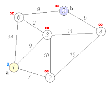
However, the assumption no longer applies if the graph contains negative edge weights. Then each section can be a shortest route between the end points, but you could improve the total distance via a longer partial path if a negative edge reduces the length of the path again. In the picture with the nodes 1, 2, 3 and 4, the Dijkstra algorithm would find the shortest way from 1 to 3 via 2, since the step to 4 has been overall than the entire upper path. However, the negative edge causes the lower path to be shorter.

after-content-x4

Algorithm in pseudocode [ Edit | Edit the source text ]

The following lines of pseudocode describe a function called Dijkstra, which receives a graph and a starting knot in the graph as input. The starting node indicates the knot from which the shortest ways to all the knots are sought. The result is a list for each knot in the previous node on the way from the start node too in indicated.

The graph consists of nodes and weighted edges, with the weight of the distance between the knots. If there is an edge between two knots, the knots are neighbors. The node currently considered in the partial step is with in referred to and is called “viewing node”. The possible, coming neighboring nodes are in the respective, upcoming intermediate examination with each in referred to as “test node”. The edge weight between viewing node in and respective test nodes in is in pseudocode as distance_ between (u, v) given.

The numerical value of distance [v] In the branch of the examination, contains the respective total removal, which the partial distances from the starting point via possible intermediate nodes and the current nodes in Until the next knot to be examined in added.

First of all, the distances and predecessors are initiated depending on the graph and start nodes. This happens in the method initialize . The actual algorithm uses a method distance_update that carries out an update of the distances if a shorter path has been found.

first function Dijkstra( Graph , The starter knot ):
 2 initialized ( Graph , The starter knot , distance [], predecessor [], Q )
 3 as long as  Q  not file: // The actual algorithm 4 in : = Knot in Q With the smallest value at a distance []
 5 remove in out of Q  // for in the shortest way is determined now 6 for each Neighbors in from in :
 7 falls  in in Q : // if not yet calculated 8 distance_update ( in , in , distance [], predecessor []) // check the distance from the start node too in  9 return predecessor[]

The initialization relies on the distances to infinity and the predecessors as unknown. Only the start node has the distance 0. The amount Q Contains the knots to which no shortest way has been found.

first Method Initialize (graph, start node, distance [], predecessor [], Q):
 2 for each node in in Graph :
 3 distance [ in ]: = infinite 4 predecessors [ in ]: = null 5 distance [ The starter knot ]: = 0
 6 Q : = All nodes in Graph

The distance from the start node to the knot in If the path is too in above in shorter than the previously known path is. Accordingly in To the predecessor of in On the shortest way.

first Method distance_update (u, v, distance [], predecessor []):
 2 alternative : = distance [ in ] + distance_ between ( in , in ) // path length from the start node to V over u 3 falls  alternative in ]:
 4 distance [ in ]: = alternative 5 predecessors [ in ]: = in

If you are only interested in the shortest way between two knots, you can Dijkstra Let the function be canceled if in = Target knot is.

The shortest way to one Target knot can now be through iteration about the predecessor determine:

first function Creation abbreviation path (target node, predecessor [])
2 Away[] : = [Target node]
3 in : = Target knot 4 as long as predecessor[ in ] not  null : // The predecessor of the start node is zero 5 in : = predecessor [ in ]
6 join in at the beginning of Away[] a
7 return Away[]

implementation [ Edit | Edit the source text ]

Knotes and edges between knots can mostly be represented by matrices or pointer structures. A pointer can also refer to the predecessor of a node. The distances of the knots can be stored in fields.

For efficient implementation, the amount is Q The knot, for which no shortest way has been found, implemented by a priority queue. The elaborate initialization takes place only once, but the repeated access is on Q more efficient. His respective distance is used as the key value for the knot, which is included in the pseudocode distance [v] is given. If the distance is shortened, partial resorting the queue is necessary.

As a data structure, a distance table or an adjenzenz matrix is available.

The following example in the programming language C ++ shows the implementation of the Dijkstra algorithm for an undemanded graph that is stored as an adjacetic list. When executing the program, the function is main Used that spend a shortest way on the console. ^[2]^[3]

Code snippet
#include #include #include #include #include #include #include #include #include using namespace std; const double maximumWeight = numeric_limits<double>::infinity(); // Konstante für das maximale Gewicht // Datentyp, der die Nachbarknoten eines Knotens definiert struct neighbor { int targetIndex; // Index des Zielknotens string name; // Name des double weight; // Gewicht der Kante neighbor(int _target, string _name, double _weight) : targetIndex(_target), name(_name), weight(_weight) { } }; // Berechnet die kürzesten Wege für den Knoten mit startIndex. Der gerichtete Graph wird als Adjazenzliste übergeben. void ComputeShortestPathsByDijkstra(int startIndex, const vector<vector<neighbor>>& adjacencyList, vector<double>& minimumDistances, vector<int>& previousVertices, map<int, string>& vertexNames) { int numberOfVertices = adjacencyList.size(); // Anzahl der Knoten // Initialisiert den Vektor für die kleinsten Abstände minimumDistances.clear(); minimumDistances.resize(numberOfVertices, maximumWeight); minimumDistances[startIndex] = 0; // Initialisiert den Vektor für die Vorgängerknoten previousVertices.clear(); previousVertices.resize(numberOfVertices, -1); set<pair<double, int>> vertexQueue; vertexQueue.insert(make_pair(minimumDistances[startIndex], startIndex)); // Warteschlange, die die Knoten des kürzesten Wegs enthält. Fügt den Startknoten hinzu. vertexNames.insert(make_pair(startIndex, vertexNames[startIndex])); // Zuordnungstabelle, die die Knoten des kürzesten Wegs enthält. Fügt den Startknoten hinzu. while (!vertexQueue.empty()) // Solange die Warteschlange nicht leer ist { double distance = vertexQueue.begin()->first; // Abstand int index = vertexQueue.begin()->second; vertexQueue.erase(vertexQueue.begin()); // Entfernt den ersten Knoten der Warteschlange const vector<neighbor>& neighbors = adjacencyList[index]; // Diese for-Schleife durchläuft alle Nachbarn des Knoten mit index for (vector<neighbor>::const_iterator neighborIterator = neighbors.begin(); neighborIterator != neighbors.end(); neighborIterator++) { int targetIndex = neighborIterator->targetIndex; // Index des Nachbarknotens string name = neighborIterator->name; // Name des Nachbarknotens double weight = neighborIterator->weight; // Abstand zum Nachbarknoten double currentDistance = distance + weight; // Abstand vom Startknoten zum Knoten mit index if (currentDistance < minimumDistances[targetIndex]) // Wenn der Abstand zum Nachbarknoten kleiner als die Länge des bisher kürzesten Wegs ist { vertexQueue.erase(make_pair(minimumDistances[targetIndex], targetIndex)); // Entfernt den Knoten aus der Warteschlange vertexNames.erase(targetIndex); // Entfernt den Namen des Knotens aus der Zuordnungstabelle minimumDistances[targetIndex] = currentDistance; // Speichert den Abstand vom Startknoten previousVertices[targetIndex] = index; // Speichert den Index des Vorgängerknotens vertexQueue.insert(make_pair(minimumDistances[targetIndex], targetIndex)); // Fügt den Knoten der Warteschlange hinzu vertexNames.insert(make_pair(targetIndex, name)); // Fügt den Namen des Knotens der Zuordnungstabelle hinzu } } } } // Gibt einen kürzesten Weg für den Knoten mit index zurück list<string> GetShortestPathTo(int index, vector<int>& previousVertices, map<int, string>& vertexNames) { list<string> path; for (; index != -1; index = previousVertices[index]) // Diese for-Schleife durchläuft den Weg { path.push_front(vertexNames[index]); // Fügt den Namen des Vorgängerknotens hinzu } return path; } // Hauptfunktion die das Programm ausführt int main() { // Initialisiert die Adjazenzliste des gerichteten Graphen mit 6 Knoten vector<vector<neighbor>> adjacencyList(6); adjacencyList[0].push_back(neighbor(1, "Knoten 1", 7)); adjacencyList[0].push_back(neighbor(2, "Knoten 2", 9)); adjacencyList[0].push_back(neighbor(5, "Knoten 5", 14)); adjacencyList[1].push_back(neighbor(0, "Knoten 0", 7)); adjacencyList[1].push_back(neighbor(2, "Knoten 2", 10)); adjacencyList[1].push_back(neighbor(3, "Knoten 3", 15)); adjacencyList[2].push_back(neighbor(0, "Knoten 0", 9)); adjacencyList[2].push_back(neighbor(1, "Knoten 1", 10)); adjacencyList[2].push_back(neighbor(3, "Knoten 3", 11)); adjacencyList[2].push_back(neighbor(5, "Knoten 5", 2)); adjacencyList[3].push_back(neighbor(1, "Knoten 1", 15)); adjacencyList[3].push_back(neighbor(2, "Knoten 2", 11)); adjacencyList[3].push_back(neighbor(4, "Knoten 4", 6)); adjacencyList[4].push_back(neighbor(3, "Knoten 3", 6)); adjacencyList[4].push_back(neighbor(5, "Knoten 5", 9)); adjacencyList[5].push_back(neighbor(0, "Knoten 0", 14)); adjacencyList[5].push_back(neighbor(2, "Knoten 2", 2)); adjacencyList[5].push_back(neighbor(4, "Knoten 4", 9)); vector<double> minimumDistances; // Vektor für die kleinsten Abstände vector<int> previousVertices; // Vektor für die Vorgängerknoten map<int, string> vertexNames; // Vektor für die Namen der Knoten ComputeShortestPathsByDijkstra(0, adjacencyList, minimumDistances, previousVertices, vertexNames); // Aufruf der Methode, die die kürzesten Wege für den Knoten 0 zurückgibt cout << "Abstand von Knoten 0 nach Knoten 4: " << minimumDistances[4] << endl; // Ausgabe auf der Konsole list<string> path = GetShortestPathTo(4, previousVertices, vertexNames); // Aufruf der Methode, die einen kürzesten Weg von Knoten 0 nach Knoten 4 zurückgibt cout << "Kürzester Weg:"; // Ausgabe auf der Konsole copy(path.begin(), path.end(), ostream_iterator<string>(cout, " ")); // Ausgabe auf der Konsole cout << endl; // Ausgabe auf der Konsole }

Code snippet

#include   #include   #include   #include 
#include 
#include 
#include 
#include 
#include 
using namespace std;

const double maximumWeight = numeric_limits<double>::infinity(); // Konstante für das maximale Gewicht

// Datentyp, der die Nachbarknoten eines Knotens definiert
struct neighbor
{
    int targetIndex; // Index des Zielknotens
    string name; // Name des 
    double weight; // Gewicht der Kante
    neighbor(int _target, string _name, double _weight) : targetIndex(_target), name(_name), weight(_weight) { }
};

// Berechnet die kürzesten Wege für den Knoten mit startIndex. Der gerichtete Graph wird als Adjazenzliste übergeben.
void ComputeShortestPathsByDijkstra(int startIndex, const vector<vector<neighbor>>& adjacencyList, vector<double>& minimumDistances, vector<int>& previousVertices, map<int, string>& vertexNames)
{
    int numberOfVertices = adjacencyList.size(); // Anzahl der Knoten
     // Initialisiert den Vektor für die kleinsten Abstände
    minimumDistances.clear();
    minimumDistances.resize(numberOfVertices, maximumWeight);
    minimumDistances[startIndex] = 0;
    // Initialisiert den Vektor für die Vorgängerknoten
    previousVertices.clear();
    previousVertices.resize(numberOfVertices, -1);
    set<pair<double, int>> vertexQueue;
    vertexQueue.insert(make_pair(minimumDistances[startIndex], startIndex)); // Warteschlange, die die Knoten des kürzesten Wegs enthält. Fügt den Startknoten hinzu.
    vertexNames.insert(make_pair(startIndex, vertexNames[startIndex])); // Zuordnungstabelle, die die Knoten des kürzesten Wegs enthält. Fügt den Startknoten hinzu.
    while (!vertexQueue.empty()) // Solange die Warteschlange nicht leer ist
    {
        double distance = vertexQueue.begin()->first; // Abstand
        int index = vertexQueue.begin()->second;
        vertexQueue.erase(vertexQueue.begin()); // Entfernt den ersten Knoten der Warteschlange
        const vector<neighbor>& neighbors = adjacencyList[index];
        // Diese for-Schleife durchläuft alle Nachbarn des Knoten mit index
        for (vector<neighbor>::const_iterator neighborIterator = neighbors.begin(); neighborIterator != neighbors.end(); neighborIterator++)
        {
            int targetIndex = neighborIterator->targetIndex; // Index des Nachbarknotens
            string name = neighborIterator->name; // Name des Nachbarknotens
            double weight = neighborIterator->weight; // Abstand zum Nachbarknoten
            double currentDistance = distance + weight; // Abstand vom Startknoten zum Knoten mit index
            if (currentDistance < minimumDistances[targetIndex]) // Wenn der Abstand zum Nachbarknoten kleiner als die Länge des bisher kürzesten Wegs ist
            {
                vertexQueue.erase(make_pair(minimumDistances[targetIndex], targetIndex)); // Entfernt den Knoten aus der Warteschlange
                vertexNames.erase(targetIndex); // Entfernt den Namen des Knotens aus der Zuordnungstabelle
                minimumDistances[targetIndex] = currentDistance; // Speichert den Abstand vom Startknoten
                previousVertices[targetIndex] = index; // Speichert den Index des Vorgängerknotens
                vertexQueue.insert(make_pair(minimumDistances[targetIndex], targetIndex)); // Fügt den Knoten der Warteschlange hinzu
                vertexNames.insert(make_pair(targetIndex, name)); // Fügt den Namen des Knotens der Zuordnungstabelle hinzu
            }
        }
    }
}

// Gibt einen kürzesten Weg für den Knoten mit index zurück
list<string> GetShortestPathTo(int index, vector<int>& previousVertices, map<int, string>& vertexNames)
{
    list<string> path;
    for (; index != -1; index = previousVertices[index]) // Diese for-Schleife durchläuft den Weg
    {
        path.push_front(vertexNames[index]); // Fügt den Namen des Vorgängerknotens hinzu
    }
    return path;
}

// Hauptfunktion die das Programm ausführt
int main()
{
    // Initialisiert die Adjazenzliste des gerichteten Graphen mit 6 Knoten
    vector<vector<neighbor>> adjacencyList(6);

    adjacencyList[0].push_back(neighbor(1, "Knoten 1", 7));
    adjacencyList[0].push_back(neighbor(2, "Knoten 2", 9));
    adjacencyList[0].push_back(neighbor(5, "Knoten 5", 14));

    adjacencyList[1].push_back(neighbor(0, "Knoten 0", 7));
    adjacencyList[1].push_back(neighbor(2, "Knoten 2", 10));
    adjacencyList[1].push_back(neighbor(3, "Knoten 3", 15));

    adjacencyList[2].push_back(neighbor(0, "Knoten 0", 9));
    adjacencyList[2].push_back(neighbor(1, "Knoten 1", 10));
    adjacencyList[2].push_back(neighbor(3, "Knoten 3", 11));
    adjacencyList[2].push_back(neighbor(5, "Knoten 5", 2));

    adjacencyList[3].push_back(neighbor(1, "Knoten 1", 15));
    adjacencyList[3].push_back(neighbor(2, "Knoten 2", 11));
    adjacencyList[3].push_back(neighbor(4, "Knoten 4", 6));

    adjacencyList[4].push_back(neighbor(3, "Knoten 3", 6));
    adjacencyList[4].push_back(neighbor(5, "Knoten 5", 9));

    adjacencyList[5].push_back(neighbor(0, "Knoten 0", 14));
    adjacencyList[5].push_back(neighbor(2, "Knoten 2", 2));
    adjacencyList[5].push_back(neighbor(4, "Knoten 4", 9));

    vector<double> minimumDistances; // Vektor für die kleinsten Abstände
    vector<int> previousVertices; // Vektor für die Vorgängerknoten
    map<int, string> vertexNames; // Vektor für die Namen der Knoten
    ComputeShortestPathsByDijkstra(0, adjacencyList, minimumDistances, previousVertices, vertexNames); // Aufruf der Methode, die die kürzesten Wege für den Knoten 0 zurückgibt
    cout << "Abstand von Knoten 0 nach Knoten 4: " << minimumDistances[4] << endl; // Ausgabe auf der Konsole
    list<string> path = GetShortestPathTo(4, previousVertices, vertexNames); // Aufruf der Methode, die einen kürzesten Weg von Knoten 0 nach Knoten 4 zurückgibt
    cout << "Kürzester Weg:"; // Ausgabe auf der Konsole
    copy(path.begin(), path.end(), ostream_iterator<string>(cout, " ")); // Ausgabe auf der Konsole
    cout << endl; // Ausgabe auf der Konsole
}

An example of the application of the dijkstra algorithm is the search for a shortest path on a map. ^[4]In the example used here you want to find a shortest path from Frankfurt to Munich in the map shown below from Germany.

The numbers on the connections between two cities indicate the distance between the two cities connected by the edge. The numbers behind the city names give the city’s determined distance to the starting knot Frankfurt ∞ stands for an unknown distance. The light gray underlaid nodes are the nodes whose distance is relaxed (i.e. a shortened if a shorter route has been found), the dark gray nodes are the ones to which the shortest way from Frankfurt is already known.

The next neighbor is selected according to the principle of a priority queue. Relaxed distances therefore require new sorting.

Example
Starting situation: non-initiated graph with start nodes Frankfurt and target node Munich
Determine distances from the start node (Frankfurt) ( Relaxation ), Rede of the priority keeper Q (1st Mannheim, 2nd Kassel, 3rd Würzburg, …)
Mannheim is the closest knot, relaxation with the neighboring node Karlsruhe, the next predecessor of Karlsruhe is now Mannheim, new sorting of Q (1st Karlsruhe, 2nd Kassel, 3. Würzburg, …)
Karlsruhe, relaxation with Augsburg, re -sorting of Q (1st Kassel, 2nd Würzburg, August 3rd, …)
The closest node to be examined is now Kassel, relaxation with Munich, new sorting of Q (1st Würzburg, 2nd Augsburg, 3rd Munich, …)
The closest node to be examined is now Würzburg, relaxation with Erfurt and Nuremberg, new sorting of Q (1st Nuremberg, 2nd Erfurt, 3rd Augsburg, 4th Munich, …)
The closest node to be examined is now Nuremberg, relaxation with Munich and Stuttgart, re -sorting of Q (1st Erfurt, 2nd Augsburg, 3. Munich, 4th Stuttgart, …)
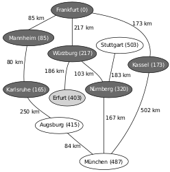
The closest node to be examined is now Erfurt, relaxation with no one, re -sorting of Q (1 Augsburg, 2nd Munich, 3rd Stuttgart, …)
The closest knot to be examined is now Augsburg, relaxation with Munich, re -sorting of Q (1st Munich, 2nd Stuttgart …)
Target node is to be examined: The shortest way to Munich is now known; Reconstruction using Creation abbreviation path () . This is: Frankfurt-Würzburg-Nuremberg-Munich.

An alternative algorithm to search for a very short path, which, on the other hand, is based on the optimality principle of Bellman, is the Floyd-Warshall algorithm. The optimality principle states that if the shortest path leads from A to C via b, the shortest path must also be the shortest path from A to B.

Another alternative algorithm is the A*algorithm, which extends the algorithm of Dijkstra with a start-up function. If this fulfills certain properties, the shortest path can be found faster.

There are various acceleration techniques for the Dijkstra algorithm, for example Arcflag.

A graph in which the tension tree calculated by the Dijkstra algorithm (starting in S) is not a minimal clamping tree of the graph.

After the end of the algorithm is in the predecessors Pi a partial span tree of the component of

{displaystyle s}

$s$ From the shortest paths of

{displaystyle s}

$s$ to all the nodes of the component that were included in the cue. However, this tree is not necessarily minimal, as the illustration shows:

May be

{displaystyle x}

$x$ A number larger 0. Minimally exciting trees are either through the edges

{displaystyle left{a,sright}}

${displaystyle left{a,sright}}$ and

{displaystyle left{a,bright}}

${displaystyle left{a,bright}}$ or

{displaystyle left{b,sright}}

${displaystyle left{b,sright}}$ and

{displaystyle left{a,bright}}

${displaystyle left{a,bright}}$ given. The total costs of a minimally exciting tree are

{displaystyle 2+x}

${displaystyle 2+x}$ . Dijkstras Algorithm delivers with starting point

{displaystyle s}

$s$ the edges

{displaystyle left{a,sright}}

${displaystyle left{a,sright}}$ and

{displaystyle left{b,sright}}

${displaystyle left{b,sright}}$ as a result. The total costs of this exciting tree are

{displaystyle 2+2x}

${displaystyle 2+2x}$ .

The algorithm from Prim or the Algorithm from Kruskal is possible with the algorithm from Prim or the Algorithm from Prim or the Algorithm.

The following assessment only applies to graphs that do not contain negative edge weights.

The term of the Dijkstra algorithm depends on the number of edges

{displaystyle |E|}

$|E|$ and the number of nodes

{displaystyle |V|}

$|V|$ . The exact time complexity depends on the data structure

{displaystyle Q}

$Q$ from in which the knots are saved.
For all implementations of

{displaystyle Q}

$Q$ is applicable:

{displaystyle O(|E|cdot T_{mathrm {dk} }+|V|cdot T_{mathrm {em} })}

whereby

{displaystyle T_{mathrm {dk} }}

${displaystyle T_{mathrm {dk} }}$ and

{displaystyle T_{mathrm {em} }}

${displaystyle T_{mathrm {em} }}$ For the complexity of the decrease-key – and extract-minimum -Perivations at

{displaystyle Q}

$Q$ stand. The simplest implementation for

{displaystyle Q}

$Q$ is a list or an array. The time complexity is

{Displaystyle o (| E |+| V |^{2}) = O (| V |^{2})}

${displaystyle O(|E|+|V|^{2})=O(|V|^{2})}$ .

Normally, you will use a priority queue here by using the nodes there as elements with their respective distant distance as a key/priority.

The optimal term for a graph

{displaystyle G=(V,E)}

$G = (V, E)$ amounts to

{Displaystyle O (| V | log (| V |)+| E |)}

${displaystyle O(|V|log(|V|)+|E|)}$ by using a Fibonacci heap for the Dijkstra algorithm. ^[5]

Route planners are a prominent example in which this algorithm can be used. The graph represents the network of traffic routes, which connects various points. We are looking for the shortest route between two points.

Some topological indices, such as the J-index of Balaban, need weighted distances between the atoms of a molecule. In these cases, weighting is the binding regulations.

Dijkstras Algorithm is also used on the Internet as a routing algorithm in the OSPF, IS-IS and OLSR protocol. The latter Optimized Link State Routing -Protocol is a version of the Link State Routing adapted to the requirements of a mobile wireless LAN. It is important for mobile ad hoc networks. The free radio networks are possible.

The Dijkstra algorithm can also be used when solving the coin problem, a number-theoretical problem that has nothing to do with graphs at first glance.

If you have enough information about the edge weights in the graph in order to be able to derive a heuristic for the costs of individual nodes, it is possible to expand Dijkstra’s algorithm to the A*algorithm. In order to calculate all the shortest paths from one knot to all other nodes in a graph, you can also use the Bellman-Ford algorithm, which can handle negative edge weights. The algorithm of Floyd and Warshall finally calculates the shortest paths of all nodes.

Thomas H Cormmen, Charles E. Leiseron, Ronald L. Rivest, Clifford Stein: Algorithms – an introduction . Oldenbourg, Munich/ Vienna 2004, ISBN 3-486-27515-1, S. 598–604 (English: Introduction to algorithms . Translated by Karen Lippert, Micaela Krieger-Hauwede).
Robert Sedgewick: Algorithms in C++ Part 5: Graph Algorithms. Indianapolis 2002, ISBN 0-201-36118-3, S. 293–3
Edsger W. Dijkstra: A note on two problems in connexion with graphs. In: Numerical Mathematics. 1, 1959, S. 269–271; ma.tum.de (PDF; 739 kB).

↑ Tobias Häberlein: Practical algorithm with python. Oldenbourg, Munich 2012, ISBN 978-3-486-71390-9, p. 162 ff.
↑ Rosetta Code: Dijkstra’s algorithm
↑ GeeksforGeeks: Dijkstra’s shortest path algorithm
↑ The Simple, Elegant Algorithm That Makes Google Maps Possible. At: VICE. Accessed on October 3, 2020.
↑ Thomas H. Cormen: Introduction to Algorithms . With press, S. 663 .

after-content-x4

Dijkstra-Algorithmus – Wikipedia Wikipedia

Informal presentation [ Edit | Edit the source text ]

Algorithm in pseudocode [ Edit | Edit the source text ]

implementation [ Edit | Edit the source text ]

Recent Posts

Recent Comments

Archives

Categories

Meta