Mason’s gain formula – Wikipedia

Mason’s gain formula (MGF) is a method for finding the transfer function of a linear signal-flow graph (SFG). The formula was derived by Samuel Jefferson Mason,^[1] whom it is also named after. MGF is an alternate method to finding the transfer function algebraically by labeling each signal, writing down the equation for how that signal depends on other signals, and then solving the multiple equations for the output signal in terms of the input signal. MGF provides a step by step method to obtain the transfer function from a SFG. Often, MGF can be determined by inspection of the SFG. The method can easily handle SFGs with many variables and loops including loops with inner loops. MGF comes up often in the context of control systems, microwave circuits and digital filters because these are often represented by SFGs.

Formula[edit]

The gain formula is as follows:

${displaystyle G={frac {y_{text{out}}}{y_{text{in}}}}={frac {sum _{k=1}^{N}{G_{k}Delta _{k}}}{Delta }}}$

${displaystyle Delta =1-sum L_{i}+sum L_{i}L_{j}-sum L_{i}L_{j}L_{k}+cdots +(-1)^{m}sum cdots +cdots }$

where:

• Δ = the determinant of the graph.
• y_in = input-node variable
• y_out = output-node variable
• G = complete gain between y_in and y_out
• N = total number of forward paths between y_in and y_out
• G_k = path gain of the kth forward path between y_in and y_out
• L_i = loop gain of each closed loop in the system
• L_iL_j = product of the loop gains of any two non-touching loops (no common nodes)
• L_iL_jL_k = product of the loop gains of any three pairwise nontouching loops
• Δ_k = the cofactor value of Δ for the k^th forward path, with the loops touching the k^th forward path removed.

Definitions^[2][edit]

• Path: a continuous set of branches traversed in the direction that they indicate.
• Forward path: A path from an input node to an output node in which no node is touched more than once.
• Loop: A path that originates and ends on the same node in which no node is touched more than once.
• Path gain: the product of the gains of all the branches in the path.
• Loop gain: the product of the gains of all the branches in the loop.

Procedure to find the solution[edit]

1. Make a list of all forward paths, and their gains, and label these G_k.
2. Make a list of all the loops and their gains, and label these L_i (for i loops). Make a list of all pairs of non-touching loops, and the products of their gains (L_iL_j). Make a list of all pairwise non-touching loops taken three at a time (L_iL_jL_k), then four at a time, and so forth, until there are no more.
3. Compute the determinant Δ and cofactors Δ_k.
4. Apply the formula.

Examples[edit]

Circuit containing two-port[edit]

Signal flow graph of a circuit containing a two port. The forward path from input to output is shown in a different color.

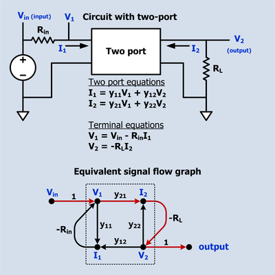
The transfer function from V_in to V₂ is desired.

There is only one forward path:

• V_in to V₁ to I₂ to V₂ with gain
  ${displaystyle G_{1}=-y_{21}R_{L},}$

  

There are three loops:

• V₁ to I₁ to V₁ with gain
  ${displaystyle L_{1}=-R_{text{in}}y_{11},}$

  

• V₂ to I₂ to V₂ with gain
  ${displaystyle L_{2}=-R_{L}y_{22},}$

  

• V₁ to I₂ to V₂ to I₁ to V₁ with gain
  ${displaystyle L_{3}=y_{21}R_{L}y_{12}R_{text{in}},}$

  

${displaystyle Delta =1-(L_{1}+L_{2}+L_{3})+(L_{1}L_{2}),}$

note: L₁ and L₂ do not touch each other whereas L₃ touches both of the other loops.

${displaystyle Delta _{1}=1,}$

note: the forward path touches all the loops so all that is left is 1.

${displaystyle G={frac {G_{1}Delta _{1}}{Delta }}={frac {-y_{21}R_{L}}{1+R_{text{in}}y_{11}+R_{L}y_{22}-y_{21}R_{L}y_{12}R_{text{in}}+R_{text{in}}y_{11}R_{L}y_{22}}},}$

Digital IIR biquad filter[edit]

The signal flow graph (SFG) for a digital infinite impulse response bi-quad filter. This SFG has three forward paths and two loops.

Digital filters are often diagramed as signal flow graphs.

There are two loops

• 
  ${displaystyle L_{1}=-a_{1}Z^{-1},}$

  

• 
  ${displaystyle L_{2}=-a_{2}Z^{-2},}$

  

${displaystyle Delta =1-(L_{1}+L_{2}),}$

Note, the two loops touch so there is no term for their product.

There are three forward paths

• 
  ${displaystyle G_{0}=b_{0},}$

  

• 
  ${displaystyle G_{1}=b_{1}Z^{-1},}$

  

• 
  ${displaystyle G_{2}=b_{2}Z^{-2},}$

  

All the forward paths touch all the loops so

${displaystyle Delta _{0}=Delta _{1}=Delta _{2}=1,}$

${displaystyle G={frac {G_{0}Delta _{0}+G_{1}Delta _{1}+G_{2}Delta _{2}}{Delta }},}$

${displaystyle G={frac {b_{0}+b_{1}Z^{-1}+b_{2}Z^{-2}}{1+a_{1}Z^{-1}+a_{2}Z^{-2}}},}$

Servo[edit]

Angular position servo and signal flow graph. θ_C = desired angle command, θ_L = actual load angle, K_P = position loop gain, V_ωC = velocity command, V_ωM = motor velocity sense voltage, K_V = velocity loop gain, V_IC = current command, V_IM = current sense voltage, K_C = current loop gain, V_A = power amplifier output voltage, V_M = effective voltage across the inductance, L_M = motor inductance, I_M = motor current, R_M = motor resistance, R_S = current sense resistance, K_M = motor torque constant (Nm/amp), T = torque, M = moment of inertia of all rotating components α = angular acceleration, ω = angular velocity, β = mechanical damping, G_M = motor back EMF constant, G_T = tachometer conversion gain constant. There is one forward path (shown in a different color) and six feedback loops. The drive shaft assumed to be stiff enough to not treat as a spring. Constants are shown in black and variables in purple.

The signal flow graph has six loops. They are:

• 
  ${displaystyle L_{0}=-{frac {beta }{sM}},}$

  

• 
  ${displaystyle L_{1}={frac {-(R_{M}+R_{S})}{sL_{M}}},}$

  

• 
  ${displaystyle L_{2}=,{frac {-G_{M}K_{M}}{s^{2}L_{M}M}}}$

  

• 
  ${displaystyle L_{3}={frac {-K_{C}R_{S}}{sL_{M}}},}$

  

• 
  ${displaystyle L_{4}={frac {-K_{V}K_{C}K_{M}G_{T}}{s^{2}L_{M}M}},}$

  

• 
  ${displaystyle L_{5}={frac {-K_{P}K_{V}K_{C}K_{M}}{s^{3}L_{M}M}},}$

  

${displaystyle Delta =1-(L_{0}+L_{1}+L_{2}+L_{3}+L_{4}+L_{5})+(L_{0}L_{1}+L_{0}L_{3}),}$

There is one forward path:

• 
  ${displaystyle g_{0}={frac {K_{P}K_{V}K_{C}K_{M}}{s^{3}L_{M}M}},}$

  

The forward path touches all the loops therefore the co-factor

And the gain from input to output is

Equivalent matrix form[edit]

Mason’s rule can be stated in a simple matrix form. Assume

is the transient matrix of the graph where

is the sum transmittance of branches from node m toward node n. Then, the gain from node m to node n of the graph is equal to

, where

${displaystyle mathbf {U} =left(mathbf {I} -mathbf {T} right)^{-1}}$

,

and

is the identity matrix.

Mason’s Rule is also particularly useful for deriving the z-domain transfer function of discrete networks that have inner feedback loops embedded within outer feedback loops (nested loops). If the discrete network can be drawn as a signal flow graph, then the application of Mason’s Rule will give that network’s z-domain H(z) transfer function.

Complexity and computational applications[edit]

Mason’s Rule can grow factorially, because the enumeration of paths in a directed graph grows dramatically. To see this consider the complete directed graph on

vertices, having an edge between every pair of vertices. There is a path form

to

for each of the

permutations of the intermediate vertices. Thus Gaussian elimination is more efficient in the general case.

Yet Mason’s rule characterizes the transfer functions of interconnected systems in a way which is simultaneously algebraic and combinatorial, allowing for general statements and other computations in algebraic systems theory. While numerous inverses occur during Gaussian elimination, Mason’s rule naturally collects these into a single quasi-inverse. General form is

${displaystyle {frac {p}{1-q}},}$

Where as described above,

is a sum of cycle products, each of which typically falls into an ideal (for example, the strictly causal operators). Fractions of this form make a subring

of the rational function field. This observation carries over to the noncommutative case,^[3] even though Mason’s rule itself must then be replaced by Riegle’s rule.

See also[edit]

References[edit]

• Bolton, W. Newnes (1998). Control Engineering Pocketbook. Oxford: Newnes.
• Van Valkenburg, M. E. (1974). Network Analysis (3rd ed.). Englewood Cliffs, NJ: Prentice-Hall.